Error-Compensating Optimizers: ECO-AdamW, ECO-Muon, and Beyond

1. Introduction

To optimize inference in production settings, we typically need to quantize the model weights first, and then do all subsequent computation in low precision. But training in low precision natively is difficult, and so we often pretrain in high precision, quantize, then fine-tune to recover any lost performance. This wastes compute and we often do not fully recover the original performance.

Error-Compensating Optimizers (ECO), on the other hand, allows the (idealized) master weights to evolve in high precision while only materializing quantized weights (Nikdan et al., 2026). This eliminates the need for a separate quantization and fine-tuning phase. The crux is that we do not need to store both the weights and momentum buffers in full precision; it would suffice to store quantized weights and ‘pull’ the quantization ’error’ back into the momentum buffer for use in the next step.

In this blog post, we shall discuss how to handle weight decay and matrix LMOs in the ECO framework.

2. ECO with weight decay

2.1. ECO for SGD with momentum and weight decay

Let $q(\cdot)$ be the quantization function, $W_t^*$ and $M_t^*$ be the (idealized) master weights and momentum, and $\widehat{W}_t$ and $M_t$ be the (materialized) quantized weights and (unquantized) momentum at step $t$. Then, the master-weight SGD update with momentum and weight decay is given by,

where $0 \leq \beta < 1, \eta > 0, \lambda \geq 0$ are the momentum, learning rate, and weight decay hyperparameters, respectively.

However, we do not want to materialize the master weights $W_t^*$, but only the quantized weights $\widehat{W}_t$, hence the ECO-style update of the form,

where $\widetilde{M}_{t+1}$ and $\widetilde{W}_{t+1}$ are intermediate variables, and $\texttt{pullback}$ is the error-compensation function that ‘pulls’ the quantization ’error’ back into the momentum buffer for use in the next step.

The challenge then is to find $\texttt{pullback}$ such that the intermediate weight variable $\widetilde{W}_t$ evolves the same as the (idealized) master weight $W_t^*$. That is, we want to enfore the invariant,

for all $t \geq 0$.

Base case: At $t=0$, we can simply initialize $W_0^* = \widetilde{W}_0 = \widehat{W}_0$ and $M_0^* = M_0 = \mathbf{0}$.

Inductive case: Assuming $W_t^* = \widetilde{W}_t$ for some $t \geq 0$, we want to find $\texttt{pullback}$ such that $W_{t+1}^* = \widetilde{W}_{t+1}$ as well. To do this, let us first combine this constraint with Equations $\eqref{eq:sgdm_w_update}$, $\eqref{eq:eco_sgdm_w_update}$, and $\eqref{eq:eco_sgdm_error}$ as follows,

Now let $\alpha_t := M_t^* - M_t$. Then combining Equations $\eqref{eq:sgdm_m_update}$, $\eqref{eq:eco_sgdm_m_update}$, and $\eqref{eq:sgdm_m_update_expanded}$ yields,

and since this holds for all $t$, we have,

Lastly, we can eliminate the dependence on $E_t$ using the heuristic $E_t \approx E_{t+1}$ observed in practice, which gives us the error-compensating momentum update rule for SGD with momentum:

where the red-colored term is the difference from Algorithm 2 in the ECO paper.

2.2. ECO for steepest descent with LMOs of the form $\texttt{LMO}(X) = g(X) X h(X)$

Steepest descent under a norm $\| \cdot \|$ with Linear Minimization Oracle (LMO), $\texttt{LMO}(X)$, has the following master-weight update rule:

and as in the previous section, the ECO-style update is given by,

Enforcing $W_t^* = \widetilde{W}_t$ as before, we have,

Now suppose we have LMOs of the form $\texttt{LMO}(X) = g(X) X h(X)$ with matrix functions $g: \mathbb{R}^{m \times n} \to \mathbb{R}^{m \times m}$ and $h: \mathbb{R}^{m \times n} \to \mathbb{R}^{n \times n}$ such that there exist $g^{-1}: \mathbb{R}^{m \times n} \to \mathbb{R}^{m \times m}$ and $h^{-1}: \mathbb{R}^{m \times n} \to \mathbb{R}^{n \times n}$ satisfying $g^{-1}(X) g(X) = I_m$ and $h(X) h^{-1}(X) = I_n$ for all $X$. Then, we can make the following approximation by freezing $g$ and $h$ (valid for small perturbations $\Delta X$ or small learning rates $\eta$ which are common in practice):

Thus, combining Equations $\eqref{eq:u_star_from_lmo}$, $\eqref{eq:u_star_from_u}$, and $\eqref{eq:lmo_approx}$, we have,

Following the same steps as before then yields,

2.2.1. ECO-Muon

Steepest descent under the RMS-to-RMS norm as in the Muon optimizer (Jordan et al., 2024) have the following LMO:

Thus, setting either $g(X) = \sqrt{\frac{m}{n}} I_m$ and $h(X) = (X^T X)^{-1/2}$ or $g(X) = I_m$ and $h(X) = \sqrt{\frac{m}{n}} (X^T X)^{-1/2}$ then gives us the error-compensating momentum update rule for Muon:

which we can compute as in Appendix A1.

2.2.2. ECO-Shampoo

The Shampoo optimizer (Gupta et al., 2018, Anil et al., 2020) instead calculates the updates as follows:

where $L_t: \mathbb{R}^{m \times m}$ and $R_t: \mathbb{R}^{n \times n}$ are the left and right preconditioners, respectively, $r \in [2, 4]$ is some root hyperparameter usually set to $r=4$, and the $\sqrt{\frac{m}{n}}$ factor ensures that the RMS-to-RMS norm of $U_t$ is approximately 1 as in Muon. Thus, setting $g(X) = \sqrt{\frac{m}{n}} L_t^{-1/r}$ and $h(X) = R_t^{-1/r}$ then yields the error-compensating momentum update rule for Shampoo:

2.2.3. ECO-PSGD

Muon computes its preconditioner instantaneously while Shampoo accumulates its left and right preconditioners over time. PSGD, on the other hand, “learns” its preconditioner(s) over time while constraining them to satisfy some criteria (Pooladzandi and Li, 2024). We focus on Muon-style PSGD which computes the update as:

where $P_t := Q_t^T Q_t$ and $Q_t \in \mathbb{R}^{n \times n}$ is some learned upper-triangular factor which we update, occasionally, with the following rule:

Setting $g(X) = \sqrt{\frac{m}{n}} I_m$ and $h(X) = P_t$ then gives us the error-compensating momentum update rule for Muon-style PSGD:

We already compute $Q_t^{-1}$ in the preconditioner update step (Equation $\eqref{eq:psgd_preconditioner_update}$), so we can reuse it here to compute $P_t^{-1}$ efficiently.

2.3. ECO for steepest descent with LMOs of the form $\texttt{LMO}(X) = X \odot h(X)$

Suppose we instead have LMOs of the form $\texttt{LMO}(X) = X \odot h(X)$, where $\odot$ is the element-wise product, and $h: \mathbb{R}^{m \times n} \to \mathbb{R}^{m \times n}$ is some matrix function such that there exists $h^{-1}: \mathbb{R}^{m \times n} \to \mathbb{R}^{m \times n}$ satisfying $h(X) \odot h^{-1}(X) = \mathbf{1}_{m \times n}$ for all $X$. Then, following the same steps as before, we have the error-compensating momentum update rule,

2.3.1. ECO-AdamW

For AdamW (Adam with (decoupled) weight decay), we have the LMO,

where $\widetilde{V}_t$ is the second moment accumulator. Thus,

where the blue-colored term is the difference from Algorithm 3 in the ECO paper.

3. Experiments [WIP]

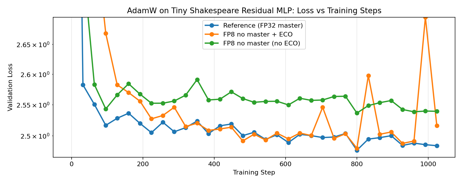
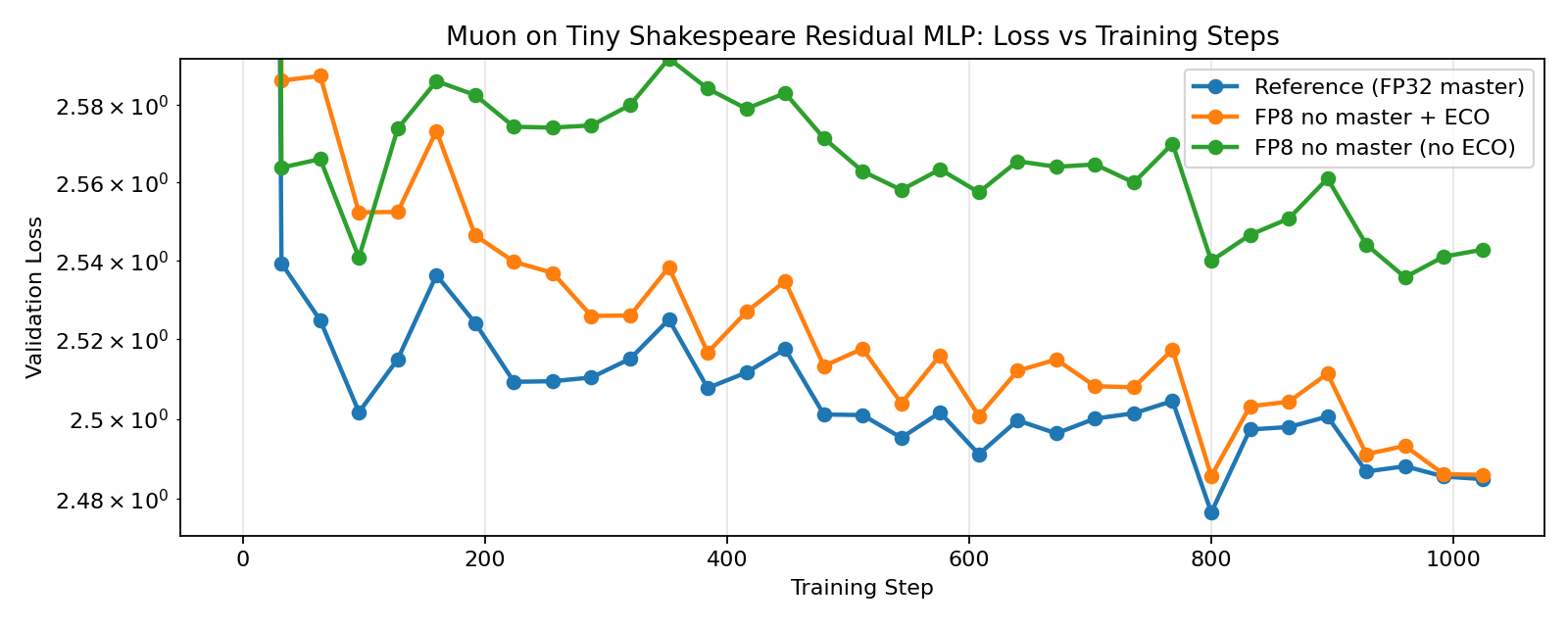
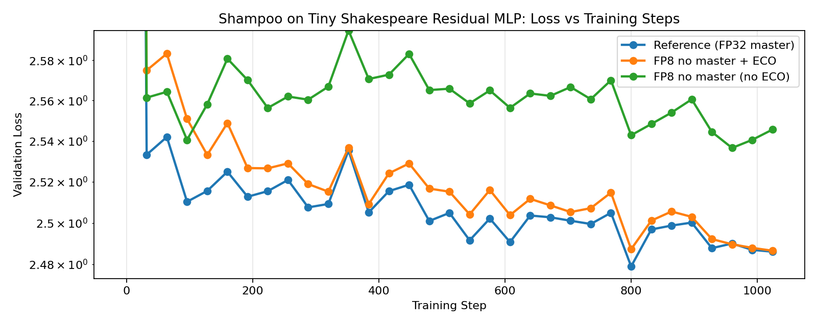
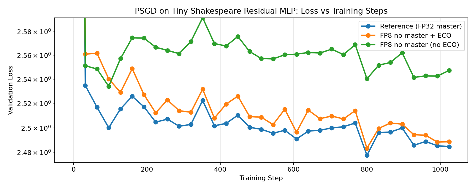
Here we train 4-layer Residual MLPs on the Tiny Shakespeare dataset with FP8 ECO-AdamW, ECO-Muon, ECO-Shampoo, and ECO-PSGD, and compare with their (still FP8) non-ECO counterparts and reference full-precision implementions. For the FP8 training runs, we quantize both the weights and activations with a straight-through estimator in the forward pass of the linear layers. Language model heads are kept in full-precision for all runs since it is the most sensitive to quantization. And Embedding layers are always optimized either by ECO-AdamW or its non-ECO counterpart since Muon/Shampoo/PSGD are only designed for linear layers. And lastly, we also match the spectral norms of the updates for Muon, Shampoo, and PSGD to that of AdamW for a more direct comparison.

Important note: these are preliminary results, and I haven’t fully tuned the hyperparameters for these runs yet.

3.1. ECO-AdamW

3.2. ECO-Muon

3.3. ECO-Shampoo

3.4. ECO-PSGD

3.5. Discussion

Our results show that ECO-AdamW, ECO-Muon, ECO-Shampoo, and ECO-PSGD closely track their full-precision counterparts, while the non-ECO versions noticeably diverge, demonstrating the effectiveness of ECO in FP8-native training without master weights. When FP8 training is enabled for all components (including the language model head), we see even more significant divergence for the non-ECO versions, while the ECO versions see only a slight increase in loss, matching the results by Nikdan et al., 2026.

How to cite

@misc{cesista2026eco,
  author = {Franz Louis Cesista},
  title = {{E}rror-{C}ompensating {O}ptimizers: {ECO}-{A}dam{W}, {ECO}-{M}uon, and Beyond},
  year = {2026},
  month = {February},
  day = {10},
  url = {https://leloykun.github.io/ponder/eco/},
}

References

1. Mahdi Nikdan, Amir Zandieh, Dan Alistarh, Vahab Mirrokni (2026). ECO: Quantized Training without Full-Precision Master Weights. URL https://arxiv.org/abs/2601.22101
2. Thomas Pethick, Wanyun Xie, Kimon Antonakopoulos, Zhenyu Zhu, Antonio Silveti-Falls, Volkan Cevher (2025). Training Deep Learning Models with Norm-Constrained LMOs. URL https://arxiv.org/abs/2502.07529
3. Keller Jordan, Yuchen Jin, Vlado Boza, Jiacheng You, Franz Cesista, Laker Newhouse, and Jeremy Bernstein (2024). Muon: An optimizer for hidden layers in neural networks. Available at: https://kellerjordan.github.io/posts/muon/
4. Rohan Anil, Vineet Gupta, Tomer Koren, Kevin Regan, Yoram Singer (2020). Scalable second order optimization for deep learning. URL https://arxiv.org/abs/2002.09018
5. Vineet Gupta, Tomer Koren, Yoram Singer (2018). Shampoo: Preconditioned Stochastic Tensor Optimization. URL https://arxiv.org/abs/1802.09568
6. Omead Pooladzandi, Xi-Lin Li (2024). Curvature-Informed SGD via General Purpose Lie-Group Preconditioners. URL https://arxiv.org/abs/2402.04553

Appendix A1. Sample implementation of ECO-Muon

# Newton-Schulz coefficients for matrix square roots
COEFS_R2: List[Tuple[float, float, float]] = [
    (8.287212018145622, -23.59588651909882, 17.300387312530923),
    (4.107059111542197, -2.9478499167379084, 0.54484310829266),
    (3.9486908534822938, -2.908902115962947, 0.5518191394370131),
    (3.3184196573706055, -2.488488024314878, 0.5100489401237208),
    (2.3006520199548186, -1.6689039845747518, 0.4188073119525678),
    (1.8913014077874002, -1.2679958271945908, 0.37680408948524996),
    (1.875, -1.25, 0.375),
]

# Muon orthogonalization coefficients.
MUON_NS_COEFFS: List[Tuple[float, float, float]] = [
    (7.2086, -15.5131, 9.0178),
    (3.9623, -2.5813, 0.4542),
    (3.9466, -2.5765, 0.4544),
    (3.8991, -2.5671, 0.4566),
    (3.7186, -2.5308, 0.4653),
    (3.1390, -2.3073, 0.4733),
    (2.1715, -1.5246, 0.3885),
    (1.8648, -1.2224, 0.3577),
]

def _abc(coefs, step: int, scale: float) -> Tuple[float, float, float]:
    a, b, c = coefs[step] if step < len(coefs) else coefs[-1]
    # For r=2: (a/scale, b/scale^3, c/scale^5).
    return a / scale, b / (scale**3), c / (scale**5)

def _orthogonalize(M: torch.Tensor, *, steps: int = 8, eps: float = 1e-6, scale: float = 1.) -> torch.Tensor:
    # Computes msign(M) = M (M^T M)^{-1/2} = UV^T
    transpose = M.shape[0] > M.shape[1]
    if transpose:
        M = M.mT
    norm = torch.linalg.norm(M, dim=(-2, -1), keepdim=True)
    M = M / (norm + eps)
    for k in range(steps)
        a, b, c = _abc(MUON_NS_COEFFS, k, scale)
        M = a * M + (b * (U := M @ M.mT) + c * (U @ U)) @ M
    if transpose:
        M = M.mT
    return M

def _matrix_sqrt(P: torch.Tensor, *, steps: int = 8, eps: float = 1e-6, scale: float = 1.01) -> torch.Tensor:
    # Computes P^{1/2}
    assert P.ndim == 2 and P.shape[0] == P.shape[1], "P must be square"
    norm = torch.linalg.norm(P, dim=(-2, -1), keepdim=True)
    if norm <= eps:
        return torch.zeros_like(P)
    Y = YZ = P / norm
    I_n = torch.eye(P.shape[0], device=P.device, dtype=P.dtype)
    for k in range(steps):
        a, b, c = _abc(COEFS_R2, k, scale)
        W = a * I_n + b * YZ + c * (YZ @ YZ)
        Y, YZ = W @ Y, (W @ W) @ YZ
    return Y * norm**0.5

def quantize(W: torch.Tensor) -> torch.Tensor:
    ...

def update(G: torch.Tensor, M: torch.Tensor, W_quantized: torch.Tensor, eta: float, beta=0.9, lamb=0.1) -> torch.Tensor:
    m, n = G.shape
    M_tilde = beta * M + (1 - beta) * G
    U = (m/n)**0.5 * _orthogonalize(M_tilde)
    W_tilde = (1 - eta * lamb) * W_quantized.to(M_tilde.dtype) - eta * U
    W_quantized_next = quantize(W_tilde)
    E = W_tilde - W_quantized_next
    # Pullback weight quantization error to momentum buffer for use in the next step.
    M_next = M_tilde + (1 - eta * lamb) / eta * (1 - 1 / beta) * (n/m)**0.5 * E @ _matrix_sqrt(M_tilde.T @ M_tilde)
    return M_next, W_quantized_next