
1. Introduction
What is “maximal update parametrization” really about? When training neural networks, we want to (1) maximally update both the weights and activations (or “features”) while (2) keeping the ‘sizes’ or norms of the weights, activations, and gradients under control. The former is so that we can train larger models with fewer resources and the latter is so that our multi-billion dollar training runs would not randomly blow up in our faces during training. Now, bounding only the weights and using only Lipschitz-continuous layers already suffice to control the Lipschitzness of the model; and consequently also controlling the activation and gradient norms. But bounding the weights (e.g. via weight decay) may also discard components of our updates which we could have allocated to more promising directions in the first place. How do we resolve this?
The crux is to consider the geometry of the space where our weights ’live in’ and do steepest descent there. We can control the weight norms by choosing a bounded manifold and using its retraction map to keep weight norms in a comfortable range. And to prevent the retraction map from discarding parts of our updates, we can enforce that the updates be in the tangent space/cone at the current point in the manifold. Finally we can also maximally update the activations by equipping the tangent spaces/cones of the manifold with the $\texttt{RMS} \to \texttt{RMS}$ induced operator norm (or the scaled Spectral norm) as discussed by Yang et al. (2024).
Thinking Machines Lab recently published a blog post following the same idea where they discussed why and how to do steepest descent on the Stiefel manifold equipped with the (scaled) Spectral norm. But constraining the weights to be in the Stiefel manifold is too tight of a constraint. For one, this halves the effective parameters of the model. We argue that merely enforcing an upper bound on the singular values (and letting them go to zero during training if need be) would suffice and may even be better as it does not harm model expressivity as much as constraining the singular values to all have the same value.
We call this Steepest Descent on the Spectral Ball, and we shall discuss how to get this done in Section 5. But on our way to solving this problem, we needed to solve subproblems such as finding an efficient and GPU/TPU-friendly way to clip the eigenvalues of a (symmetric) matrix in Section 2, and numerically stable methods to compute projectors to eigenbases and singular subspaces in Section 3.2.1, Section 4.1.1, and Section 5.1.3. With the same tools, we also managed to solve the Steepest Descent problem on the Positive Definite Cone in Section 3 and on the Convex Spectrahedron in Section 4. Finally, in Section 6 we demonstrate that learning rate transfer (and probably also transfer of other hyperparameters) comes naturally when doing steepest descent on such manifolds.
2. Eigenvalue Clipping
In a previous blog post Ponder: Fast, Numerically Stable, and Auto-Differentiable Spectral Clipping via Newton-Schulz Iteration, we discussed a novel method for clipping singular values of a matrix without the use of expensive singular value decompositions (SVDs). This is useful in deep learning for controlling weight norms, stabilizing training, and potentially enabling more aggressive low-precision training. Following the same technique, we can also clip the eigenvalues of a (symmetric) matrix efficiently. This can be used to efficiently project matrices onto the positive semidefinite cone, which is useful in e.g. finance and quantum mechanics where some equations require matrices to be positive semidefinite.
I have previously communicated this technique to the authors of Ponder: Factorization-free Orthogonal Projection onto the Positive Semidefinite Cone with Composite Polynomial Filtering as I mistakenly thought their method for projecting onto the positive semidefinite cone was a special case of my prior work. This work, however, does generalize their technique. I recommend reading their paper!
For now, we limit ourselves to symmetric matrices $W \in \mathbb{S}^{n}$ where $\mathbb{S}^{n} = \{W \in \mathbb{R}^{n \times n} | W = W^T\}$ is the set of all $n \times n$ real symmetric matrices. Symmetric matrices have real eigenvalues and can be diagonalized by an orthogonal matrix. We define Eigenvalue Clipping as follows:
Definition 1 (Eigenvalue Clipping). Let $W \in \mathbb{S}^{n}$ be a symmetric matrix and $W = Q \Lambda Q^T$ be its eigenvalue decomposition where $\Lambda = \text{diag}(\lambda_1, \ldots, \lambda_n)$ are the eigenvalues of $W$, $\lambda_i \in \mathbb{R}$ for all $i$, and $Q^T Q = I$. Then we define Eigenvalue Clipping as the following matrix function $\texttt{eig\_clip}_{[\lambda_{min}, \lambda_{max}]}: \mathbb{S}^{n} \to \mathbb{S}^{n}$,
$$\begin{equation}\texttt{eig\_clip}_{[\lambda_{min}, \lambda_{max}]}(W) = Q \texttt{clip}_{[\lambda_{min}, \lambda_{max}]}(\Lambda) Q^T\label{1}\end{equation}$$where $\lambda_{min}, \lambda_{max} \in (-\infty, \infty)$ are hyperparameters that control the minimum and maximum attainable eigenvalues of the resulting matrix and $\texttt{clip}_{[\alpha, \beta]}: \mathbb{R} \to \mathbb{R}$ is applied element-wise on the eigenvalues of $W$,
$$\begin{equation}\texttt{clip}_{[\alpha, \beta]}(x) = \begin{cases} \alpha & \texttt{if } x < \alpha \\ x & \texttt{if } \alpha \leq x \leq \beta \\ \beta & \texttt{if } \beta < x \end{cases}\end{equation}$$where $\alpha, \beta \in \mathbb{R} \cup \{-\infty, \infty\}$ and $\alpha \leq \beta$.
The naive implementation of this requires computing the eigenvalue decomposition of $W$, which is computationally expensive and requires high numerical precision (typically float32). Instead, we make use of the GPU/TPU-friendly method to compute the matrix sign function $\texttt{msign}$ by Jordan et al. (2024) and the following identity from the previous blog post:
Proposition 2 (Computing $\texttt{clip}$ via $\texttt{sign}$). Let $\alpha, \beta \in \mathbb{R} \cup \{-\infty, \infty\}$ and $\texttt{clip}: \mathbb{R} \to \mathbb{R}$ be the clipping function defined in Definition 1. Then,
$$\begin{equation}\texttt{clip}_{[\alpha, \beta]}(x) = \frac{\alpha + \beta + (\alpha - x)\texttt{sign}(\alpha - x) - (\beta - x)\texttt{sign}(\beta - x)}{2}\label{4}\end{equation}$$
2.1 Lifting to matrix form
We can lift Equation 3 to matrix form as follows:
$$\begin{align} \texttt{eig\_clip}_{[\alpha, \beta]}(W) &= Q \texttt{clip}_{[\alpha, \beta]}(\Lambda) Q^T\nonumber\\ &= Q \frac{(\alpha + \beta) I + (\alpha I - \Lambda)\texttt{sign}(\alpha I - \Lambda) - (\beta I - \Lambda)\texttt{sign}(\beta I - \Lambda)}{2} Q^T\nonumber\\ &= \frac{1}{2} [(\alpha + \beta) QQ^T\nonumber\\ &\qquad+ Q (\alpha I - \Lambda ) \texttt{sign}(\alpha I - \Lambda) Q^T\nonumber\\ &\qquad- Q (\beta I - \Lambda ) \texttt{sign}(\beta I - \Lambda) Q^T]\nonumber\\ &= \frac{1}{2} [(\alpha + \beta) I\nonumber\\ &\qquad+ Q (\alpha I - \Lambda ) (Q^T Q) \texttt{sign}(\alpha I - \Lambda) Q^T\nonumber\\ &\qquad- Q (\beta I - \Lambda ) (Q^T Q) \texttt{sign}(\beta I - \Lambda) Q^T]\nonumber\\ \texttt{eig\_clip}_{[\alpha, \beta]}(W) &= \frac{1}{2} [(\alpha + \beta) I \nonumber \\ &\qquad+ (\alpha I - W ) \texttt{msign}(\alpha I - W) \nonumber \\ &\qquad- (\beta I - W ) \texttt{msign}(\beta I - W)] \end{align} $$which we can implement in JAX as follows:
def sym(W: jax.Array) -> jax.Array:
    return (W + W.T) / 2

def eig_clip(W: jax.Array, alpha: float=-1., beta: float=1.) -> jax.Array:
    assert W.shape[0] == W.shape[1], "W must be square"
    W = sym(W)
    I = jnp.eye(W.shape[0], dtype=W.dtype)
    result = (1/2) * (
        (alpha + beta) * I
        + (alpha * I - W) @ _orthogonalize(alpha * I - W)
        - (beta * I - W) @ _orthogonalize(beta * I - W)
    )
    return sym(result)
2.2 Eigenvalue ReLU and orthogonal projection onto the positive semidefinite cone
Suppose we want to bound the eigenvalues of $W$ from below by a minimum value $\alpha$. For $\alpha = 0$, this is equivalent to projecting $W$ onto the positive semidefinite cone which is useful in e.g. finance and quantum mechanics where objects are typically required to be positive semidefinite. We can do this by setting $\beta = +\infty$ in Equation 3:
$$\begin{align} \texttt{clip}_{[\alpha, \infty]}(x) &= \lim_{\beta \to \infty}\frac{\alpha + \beta + (\alpha - x)\texttt{sign}(\alpha - x) - (\beta - x)\texttt{sign}(\beta - x)}{2}\nonumber\\ &= \frac{\alpha + \cancel{\beta} + (\alpha - x)\texttt{sign}(\alpha - x) - (\cancel{\beta} - x)}{2}\nonumber\\ \texttt{clip}_{[\alpha, \infty]}(x) &= \frac{\alpha + x + (\alpha - x)\texttt{sign}(\alpha - x)}{2} \end{align}$$Lifting this to matrix form yields,
$$\begin{align} \texttt{eig\_relu}_\alpha(W) &= \texttt{eig\_clip}_{[\alpha, \infty]}(W)\nonumber\\ &= Q \texttt{clip}_{[\alpha, \infty]}(\Lambda) Q^T\nonumber\\ \texttt{eig\_relu}_\alpha(W) &= \frac{1}{2} [\alpha I + W + (\alpha I - W) \texttt{msign}(\alpha I - W)] \end{align}$$which we can implement in JAX as follows:
def eig_relu(W: jax.Array, alpha: float=0.) -> jax.Array:
    W = sym(W)
    I = jnp.eye(W.shape[0], dtype=W.dtype)
    result = (1/2) * (alpha * I + W + (alpha * I - W) @ _orthogonalize(alpha * I - W))
    return sym(result)
For the orthogonal projection onto the positive semidefinite cone, we set $\alpha = 0$:
$$\begin{align} \texttt{proj\_psd}(W) &= \texttt{eig\_relu}_0(W) \nonumber \\ &= \frac{1}{2} [0 + W + (0 - W) \texttt{msign}(0 - W)] \nonumber \\ \texttt{proj\_psd}(W) &= \frac{1}{2} [W + W \texttt{msign}(W)]. \end{align}$$The last equality follows from $\texttt{msign}(-W) = -\texttt{msign}(W)$. We can then implement this in JAX as follows:
def proj_psd(W: jax.Array) -> jax.Array:
    W = sym(W)
    return sym((1/2) * (W + W @ _orthogonalize(W)))
2.3 Eigenvalue Hardcapping and orthogonal projection onto the negative semidefinite cone
Suppose we have symmetric matrices $W$ as weights in a neural network and we want to guarantee that the weights do not blow up during training. We can do this by capping the eigenvalues of $W$ to a maximum value $\beta$ after each gradient update. To do this, we can set $\alpha = -\infty$ in Equation 3:
$$\begin{align} \texttt{clip}_{[-\infty, \beta]}(x) &= \lim_{\alpha \to -\infty}\frac{\alpha + \beta + (\alpha - x)\texttt{sign}(\alpha - x) - (\beta - x)\texttt{sign}(\beta - x)}{2}\nonumber\\ &= \frac{\cancel{\alpha} + \beta - \cancel{\alpha} + x - (\beta - x)\texttt{sign}(\beta - x)}{2}\nonumber\\ \texttt{clip}_{[-\infty, \beta]}(x) &= \frac{\beta + x - (\beta - x)\texttt{sign}(\beta - x)}{2} \end{align}$$Lifting this to matrix form yields,
$$\begin{align} \texttt{eig\_hardcap}_\beta(W) &= \texttt{eig\_clip}_{[-\infty, \beta]}(W) \nonumber\\ &= Q \texttt{clip}_{[-\infty, \beta]}(\Lambda) Q^T \nonumber\\ \texttt{eig\_hardcap}_\beta(W) &= \frac{1}{2} [\beta I + W - (\beta I - W) \texttt{msign}(\beta I - W)] \end{align}$$which we can implement in JAX as follows:
def eig_hardcap(W: jax.Array, beta: float=1.) -> jax.Array:
    W = sym(W)
    I = jnp.eye(W.shape[0], dtype=W.dtype)
    result = (1/2) * (beta * I + W - (beta * I - W) @ _orthogonalize(beta * I - W))
    return sym(result)
For the orthogonal projection onto the negative semidefinite cone, we set $\beta = 0$:
$$\begin{align} \texttt{proj\_nsd}(W) &= \texttt{eig\_hardcap}_0(W) \nonumber \\ &= \frac{1}{2} [0 + W - (0 - W) \texttt{msign}(0 - W)] \nonumber \\ \texttt{proj\_nsd}(W) &= \frac{1}{2} [W - W \texttt{msign}(W)] \\ \end{align}$$which we can implement in JAX as follows:
def proj_nsd(W: jax.Array) -> jax.Array:
    W = sym(W)
    return sym((1/2) * (W - W @ _orthogonalize(W)))
2.4. Stepfun

Stepfun applies the step function on the singular values/eigenvalues of a matrix. As we will discuss in the next sections, this would be useful for e.g. filtering or “picking out” eigenbasis vectors corresponding to eigenvalues in a certain range in a numerically stable way.
You (2025) first devised a implementation for the rectangular case requiring only matrix multiplications. But as can be seen in the figure above, when applied to the symmetric matrix case, it (1) also acts symmetrically to the negative eigenvalues which is not what we want, and (2) requires two (expensive) $\texttt{msign}$ calls. But a simple modification fixes both issues,
$$\begin{align} \texttt{eig\_stepfun}_{\alpha}(X) &= Q \texttt{step}(\Lambda) Q^T \nonumber \\ &= Q \frac{I + \texttt{sign}(\Lambda - \alpha I)}{2} Q^T \nonumber \\ &= \frac{1}{2}[QQ^T + Q \texttt{sign}(\Lambda - \alpha I) Q^T] \nonumber \\ &= \frac{1}{2}[I + \texttt{msign}(Q(\Lambda - \alpha I) Q^T)] \nonumber \\ \texttt{eig\_stepfun}_{\alpha}(X) &= \frac{1}{2}[I + \texttt{msign}(X - \alpha I)] \end{align}$$As can be seen in the figure above, this implementation applies the step function properly and only requires one $\texttt{msign}$ call.
We can implement this in JAX as follows:
def eig_stepfun(X: jax.Array, alpha=0.) -> jax.Array:
    I = jnp.eye(X.shape[0], dtype=X.dtype)
    return (I + _orthogonalize(X - alpha * I)) / 2.
3. Steepest descent on the PSD cone
3.1. Problem setup
Suppose we want to do steepest descent on the PSD cone under a norm $\|\cdot\|$ chosen a priori. That is, we want to do first-order optimization where we constrain our weights to be positive semidefinite and our weight updates to have bounded norm. As we previously discussed in Ponder: Heuristic Solutions for Steepest Descent on the Stiefel Manifold, we can do this as follows:
- Let $W_t \in \mathcal{M}$ be the ‘weight’ parameter at time step $t$. Compute the “raw gradient” $G_t = \nabla f(W_t)$ via e.g. backpropagation.
- Compute a ‘optimal’ descent direction $A^* \in T_{W_t} \mathcal{M}$ under the norm in the tangent space at $W_t$, $$\begin{equation} A^* = \arg\min_{A \in \mathbb{R}^{m \times n}} \langle G, A \rangle \quad \text{ s.t. } \quad \| A \|_{W_t} \leq \eta,\quad A \in T_{W_t}\mathcal{M}, \end{equation}$$ where $\eta > 0$ is the learning rate.
- Update the weight in the direction of $A^*$, $$\widetilde{W}_{t+1} \leftarrow W_t + A^*.$$ Note that $\widetilde{W}_{t+1}$ may not be on the manifold $\mathcal{M}$. And so,
- Retract the result back to the manifold via a retraction map $W_{t+1} \leftarrow \texttt{retract}_{\mathcal{M}}(\widetilde{W}_{t+1})$.
In our case, the manifold is the PSD cone, $\mathcal{M} := \mathbb{S}^n_{+} = \{W \in \mathbb{S}^n : W \succeq 0\}$. And so, we use the $\texttt{proj\_psd}$ function defined in Section 2.2 as our retraction map.
$$\texttt{retract}_{\mathbb{S}^n_{+}} := \texttt{proj\_psd} = \texttt{eig\_relu}_0.$$To find an ‘optimal’ descent direction $A^*$, we can, in some cases, use known Linear Minimization Oracles (LMOs) (Pethick et al., 2025). Or, as we discussed in Ponder: Steepest Descent on Finsler-Structured (Matrix) Manifolds, we can compute an ‘optimal’ descent direction $A^*$ via two orthogonal projection functions: (i) the projection onto the norm ball, $\texttt{proj}_{\| \cdot \|_{W_t} \leq \eta}$, and (ii) the projection onto the tangent space at $W_t$, $\texttt{proj}_{T_{W_t}\mathcal{M}}$.
If we choose the Frobenius norm, then the projection onto the norm ball is simply,
$$\texttt{proj}_{\| \cdot \|_F \leq \eta}(X) := \begin{cases} \frac{\eta}{\| X \|_F} X & \text{if } \| X \|_F > \eta \\ X & \text{otherwise} \end{cases}$$Alternatively, we can also choose to do steepest descent under the $2 \to 2$ induced operator norm. As to why we might want to do this, you need to binge-read my previous blog posts. In short, controlling the $2 \to 2$ induced operator norm of our weights allows us to control the Lipschitzness of our model which has been shown to improve robustness, generalization, and training stability. In this case, we can use the eigenvalue clipping function defined in Section 2.1 to do the projection onto the Spectral norm ball,
$$\texttt{proj}_{\| \cdot \|_{2 \to 2} \leq \eta} := \texttt{eig\_clip}_{[-\eta,\eta]}.$$The tricky part is the projection onto the tangent space/cone at $W_{t} \in \mathbb{S}^n_{+}$, $\texttt{proj}_{T_{W_{t}}\mathbb{S}^n_{+}}$.
3.2. Projection onto the tangent space/cone at a point on the PSD cone
Special Case: $W_{t}$ is an interior point of the PSD cone. That is, $W_{t} \in \mathbb{S}^n_{++} \subset \mathbb{S}^n_{+}$ or, equivalently, $W_{t} \succ 0$. Then the tangent space is the entire space of symmetric matrices,
$$T_{W_{t}} \mathbb{S}^n_{++} = \mathbb{S}^n.$$And the projection onto the tangent space is simply the symmetrization operation $\texttt{sym}(X) = (X + X^T)/2$,
$$\texttt{proj}_{T_{W_{t}}\mathbb{S}^n_{++}} = \texttt{sym}.$$General Case: For any $W_{t} \in \mathbb{S}^n_{+}$, we may no longer have a tangent space but rather a tangent cone (that is, if $H \in T_{W_{t}} \mathbb{S}^n_{+}$, then $-H$ may not be in $T_{W_{t}} \mathbb{S}^n_{+}$). And thus, we need to be careful with the directions of our inputs to the projection map. The tangent cone at $W_{t} \in \mathbb{S}^n_{+}$ is given by,
$$T_{W_{t}} \mathbb{S}^n_{+} = \{ H \in \mathbb{S}^n : \underbrace{U_0^T H U_0 \succeq 0}_{\text{don't go below 0}} \}$$where $U_0 \in \mathbb{R}^{m \times (n-r)}$ is the orthonormal basis for the null space of $W_{t}$ and $r = \texttt{rank}(W_t)$. Note that if $W_{t}$ is full rank (and therefore positive definite), then $U_0 = 0$ and we recover the special case above.
Let $\widehat{X} := \texttt{sym}(X)$, $U = \begin{bmatrix} U_{r} & U_0 \end{bmatrix}$ be the eigenbasis of $W_t$, and $P_0 = U_0 U_0^T$ be the projector onto the null space of $W_{t}$. The projection onto the tangent cone at $W_{t} \in \mathbb{S}^n_{+}$ is given by,
$$\begin{align} \texttt{proj}_{T_{W_{t}}\mathbb{S}^n_{+}}(X) &= \arg\min_{H \in T_{W_{t}}\mathbb{S}^n_{+}} \| H - X \|_F^2 \nonumber \\ &= \arg\min_{H \in T_{W_{t}}\mathbb{S}^n_{+}} \| H - (\texttt{sym}(X) + \texttt{skew}(X)) \|_F^2 \nonumber \\ &= \arg\min_{H \in T_{W_{t}}\mathbb{S}^n_{+}} \| H - \texttt{sym}(X) \|_F^2 \nonumber \\ &\qquad\qquad\qquad\quad- 2\underbrace{\langle \underbrace{H - \texttt{sym}(X)}_{\text{symmetric}}, \texttt{skew}(X) \rangle}_{=0} + \underbrace{\cancel{\| \texttt{skew}(X) \|_F^2}}_{\text{constant}} \nonumber \\ &= \arg\min_{H \in T_{W_{t}}\mathbb{S}^n_{+}} \| H - \widehat{X} \|_F^2 \nonumber \\ &= U \left[ \arg\min_{H \in T_{W_{t}}\mathbb{S}^n_{+}} \| U^T (H - \widehat{X}) U \|_F^2 \right] U^T \nonumber \\ &= U \left[ \arg\min_{H \in T_{W_{t}}\mathbb{S}^n_{+}} \left\| \begin{bmatrix} U_{r}^T (H - \widehat{X}) U_{r} & U_{r}^T (H - \widehat{X}) U_0 \\ U_0^T (H - \widehat{X}) U_{r} & U_0^T (H - \widehat{X}) U_0 \end{bmatrix} \right\|_F^2 \right] U^T \nonumber \\ &= U \begin{bmatrix} U_{r}^T \widehat{X} U_{r} & U_{r}^T \widehat{X} U_0 \\ U_0^T \widehat{X} U_{r} & (U_0^T \widehat{X} U_0)_{+} \end{bmatrix} U^T \qquad\text{since } U_0^T H_0 U_0 \succeq 0 \nonumber \\ &= U \begin{bmatrix} U_{r}^T \widehat{X} U_{r} & U_{r}^T \widehat{X} U_0 \\ U_0^T \widehat{X} U_{r} & U_0^T \widehat{X} U_0 - (U_0^T \widehat{X} U_0)_{-} \end{bmatrix} U^T \nonumber \\ &= \widehat{X} - U_0 (U_0^T \widehat{X} U_0)_{-} U_0^T \nonumber \\ &= \widehat{X} - (U_0 U_0^T \widehat{X} U_0 U_0^T)_{-} \nonumber \\ \texttt{proj}_{T_{W_{t}}\mathbb{S}^n_{+}}(X) &= \widehat{X} - \texttt{proj\_nsd}(P_0 \widehat{X} P_0) \end{align}$$where the fifth equality follows from $I = UU^T$ and the orthogonal invariance of the Frobenius norm, and the second-to-last equality is from the similarity-equivariance of matrix functions that acts entrywise on the eigenvalues/singular values.
In words,
We first symmetrize the input $X$ into $\widehat{X}$ then we subtract the negative eigenvalues of the projection of $\widehat{X}$ onto the null space of $W_{t}$.
3.2.1. Numerically stable computation of the null space projector
Intuitively, to construct the null space projector $P_0$, we can “select” from $Q$ the eigenvectors corresponding to the zero eigenvalues of $W_{t}$ as follows,
$$\begin{align} P_0 &= Q (\mathcal{i}_{(\sigma_i = 0)}(\Sigma)) Q^T \nonumber \\ &\approx Q (\mathcal{i}_{(-\epsilon < \sigma_i < \epsilon)}(\Sigma)) Q^T && \text{for small } \epsilon > 0 \nonumber \\ &= Q (\mathcal{i}_{(\sigma_i < \epsilon)}(\Sigma)) Q^T && \text{since } W \text{ is PSD}\nonumber \\ &= Q (1 - \texttt{step}(\Sigma, \epsilon)) Q^T \nonumber \\ &= I - \texttt{eig\_stepfun}(W, \epsilon) \end{align}$$where the second line is a relaxation to handle numerical precision issues.
Taking everything together yields,
@partial(jax.jit, static_argnames=("tol",))
def project_to_tangent_psd(W: jax.Array, X: jax.Array, tol=1e-3) -> jax.Array:
    P0 = jnp.eye(W.shape[0], dtype=W.dtype) - eig_stepfun(W, tol)
    return jax.lax.cond(
        jnp.rint(jnp.trace(P0)) == 0,
        lambda: sym(X),  # W is an interior point, so tangent space is all symmetric matrices
        lambda: sym((X_ := sym(X)) - proj_nsd(P0 @ X_ @ P0)),
    )
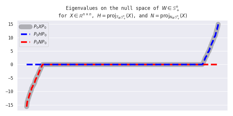
3.2.2. Sanity check
For $W_{t} \in \mathbb{S}^n_{+}$ and $X \in \mathbb{R}^{n \times n}$ initialized as follows, Let $H := \texttt{proj}_{T_{W_{t}}\mathbb{S}^n_{+}}(X)$ and $N = X - H$. Then we have, This shows that $H \in T_{W_{t}}\mathbb{S}^n_{+}$ and $N \in (T_{W_{t}}\mathbb{S}^n_{+})^\perp$ as desired.Show contents of 3.2.2. Sanity check
dim = 768
nullity = 128
keys = jax.random.split(jax.random.PRNGKey(0), 2)

W = jax.random.normal(keys[0], (dim, dim))
X = jax.random.normal(keys[1], (dim, dim))

W = sym(W @ W.T)
lam, Q = jnp.linalg.eigh(W)
lam = lam.at[:nullity].set(0)
W = Q @ jnp.diag(lam) @ Q.T
property value range of eigenvalues of $P_0 X P_0$ $[-15.67, 14.96]$ range of eigenvalues of $P_0 H P_0$ $[0.00, 14.96]$ range of eigenvalues of $P_0 N P_0$ $[-15.67, 0.00]$ alignment of $H$ to $W$ relative to the alignment of $X$: $\langle W, H \rangle / \langle W, X \rangle$ $100$% alignment of $N$ to $W$: $\langle W, N \rangle / \langle W, W \rangle$ $0$%
3.3. Update rule for steepest descent on the PSD cone
We now have all the necessary components to do steepest descent under any norm on the PSD cone.
3.3.1. Special case: $W_t$ is an interior point of the PSD cone
As we discussed in the previous section, if $W_t$ is full rank, then the tangent space at that point is simply the space of all symmetric matrices. An interesting coincidence is that Linear Minimization Oracles (LMOs) for common norms derived for the case without the tangency constraint preserve symmetry.
| Norm | LMO | preserves symmetry? |
|---|---|---|
| Frobenius norm | $X \to \frac{1}{\| X \|_F} X$ | Yes |
| $\| \cdot \|_{2 \to 2}$ | $X \to \texttt{msign}(X)$ | Yes |
Therefore, it would suffice to symmetrize the “raw gradient” $G_t$ first and then apply the LMO. This guarantees that our updates are indeed on-tangent and maximal (via theory behind LMOs). Our update rule would then be,
$$\begin{align} W_{t+1} &= \texttt{proj\_psd}\left(W_{t} + \texttt{LMO}_{\| \cdot \|_{W_t} \leq \eta}(\texttt{sym}(-G_t)) \right) \end{align}$$3.3.2. General case
In general, LMOs derived for the case without the tangency constraint often ‘send’ its output off-tangent. An example we discussed in previous blog post is $\texttt{msign}$ and the Stiefel manifold. In such cases, we can use either of the following two methods to compute an ‘optimal’ descent direction $A^*$:
- A heuristic solution such as the one discussed in Ponder: Heuristic Solutions for Steepest Descent on the Stiefel Manifold where we iteratively apply the projection onto the tangent space and the LMO until convergence. That is, $$\begin{align} W_{t+1} &= \texttt{proj\_psd}\left(W_{t} + \left(\texttt{LMO}_{\|\cdot\|_{W_t} \leq \eta} \circ \texttt{proj}_{T_{W_{t}}\mathbb{S}^n_{+}} \right)^K (-G_t) \right) \end{align}$$ for some integer $K \geq 1$ denoting the number of iterations (typically, $K = 4$ to $8$ suffices; but the iteration can be terminated upon convergence).
- An exact solution such as the primal-dual hybrid gradient method, $\texttt{pdhg}$, we discussed in Ponder: Steepest Descent on Finsler-Structured (Matrix) Manifolds, $$\begin{align} W_{t+1} &= \texttt{proj\_psd}(W_{t} + \texttt{pdhg}(-G_t, \texttt{proj}_{\| \cdot \|_{W_t} \leq \eta}, \texttt{proj}_{T_{W_{t}}\mathbb{S}^n_{+}})) \end{align}$$ We can also speed up PDHG by warm-starting the initial iterate $A^0$ with the heuristic above or the solution from the previous time step $A^*_{t-1}$ (in theory, the solutions should not drift too much between time steps if we accumulate the gradients with a momentum rule).
Voilà, we now have an efficient, factorization-free, and GPU/TPU-friendly method for doing steepest descent on the PSD cone under any norm.
4. Steepest descent on the Convex Spectrahedron
Suppose we want to constrain our weights to have eigenvalues bounded within some range $[\alpha, \beta] \subseteq \mathbb{R}$. That is, we “place” our weights on the Convex Spectrahedron,
$$\mathcal{K}_{[\alpha, \beta]} := \{W \in \mathbb{S}^n : \alpha I \preceq W \preceq \beta I\},\qquad(\alpha < \beta)$$and do steepest descent there under some norm chosen a priori. For the retraction map, we can use the eigenvalue clipping function defined in Section 2.1,
$$\texttt{retract}_{\mathcal{K}_{[\alpha, \beta]}} := \texttt{eig\_clip}_{[\alpha,\beta]}.$$4.1. Projection onto the tangent space/cone at a point on the Convex Spectrahedron
The tangent cone at $W_t \in \mathcal{K}_{[\alpha, \beta]}$ is generally given by,
$$T_{W_t} \mathcal{K}_{[\alpha, \beta]} = \{ H \in \mathbb{S}^n : \underbrace{U_{\alpha}^T H U_{\alpha} \succeq 0}_{\text{don\'t go below } \alpha}, \underbrace{U_{\beta}^T H U_{\beta} \preceq 0}_{\text{don\'t go above } \beta} \}$$where $U_{\alpha}$ and $U_{\beta}$ are the orthonormal bases for the $\alpha$- and $\beta$-eigenspaces of $W_t$, respectively. If $W_t$ is an interior point, that is, $\alpha I \prec W_t \prec \beta I$, then $U_\alpha = U_\beta = 0$ and the tangent space is simply the space of symmetric matrices, $T_{W_t} \mathcal{K}_{(\alpha, \beta)} = \mathbb{S}^n$.
Let $\widehat{X} := \texttt{sym}(X)$, $U := \begin{bmatrix} U_{\beta} & U_{\widetilde{r}} & U_{\alpha} \end{bmatrix}$ be the eigenbasis of $W_{t}$, and $P_\alpha := U_{\alpha}U_{\alpha}^T, P_\beta := U_{\beta}U_{\beta}^T$ be the projectors onto the $\alpha$- and $\beta$-eigenspaces of $W_t$, respectively. Then, following the strategy we discussed in Section 3.2, the projection onto the tangent cone at $W_t \in \mathcal{K}_{[\alpha, \beta]}$ is given by,
$$\begin{align} \texttt{proj}_{T_{W_t}\mathcal{K}_{[\alpha, \beta]}}(X) &= \arg\min_{H \in T_{W_{t}}\mathcal{K}_{[\alpha, \beta]}} \| H - X \|_F^2 \nonumber \\ &= \arg\min_{H \in T_{W_{t}}\mathcal{K}_{[\alpha, \beta]}} \| H - \widehat{X} \|_F^2 + \cancel{\text{constant}} \nonumber \\ &= U \left[ \arg\min_{H \in T_{W_{t}}\mathcal{K}_{[\alpha, \beta]}} \| U^T (H - \widehat{X}) U \|_F^2 \right] U^T \nonumber \\ &= U \begin{bmatrix} (U_{\beta}^T \widehat{X} U_{\beta})_{-} & U_{\beta}^T \widehat{X} U_{\widetilde{r}} & U_{\beta}^T \widehat{X} U_{\alpha} \\ U_{\widetilde{r}}^T \widehat{X} U_{\beta} & U_{\widetilde{r}}^T \widehat{X} U_{\widetilde{r}} & U_{\widetilde{r}}^T \widehat{X} U_{\alpha} \\ U_{\alpha}^T \widehat{X} U_{\beta} & U_{\alpha}^T \widehat{X} U_{\widetilde{r}} & (U_{\alpha}^T \widehat{X} U_{\alpha})_{+} \end{bmatrix} U^T \qquad\text{since}\quad \begin{matrix} U_{\alpha}^T H_0 U_{\alpha} \succeq 0 \\ U_{\beta}^T H_0 U_{\beta} \preceq 0 \end{matrix} \nonumber \\ &= U \begin{bmatrix} U_{\beta}^T \widehat{X} U_{\beta} - (U_{\beta}^T \widehat{X} U_{\beta})_{+} & U_{\beta}^T \widehat{X} U_{\widetilde{r}} & U_{\beta}^T \widehat{X} U_{\alpha} \\ U_{\widetilde{r}}^T \widehat{X} U_{\beta} & U_{\widetilde{r}}^T \widehat{X} U_{\widetilde{r}} & U_{\widetilde{r}}^T \widehat{X} U_{\alpha} \\ U_{\alpha}^T \widehat{X} U_{\beta} & U_{\alpha}^T \widehat{X} U_{\widetilde{r}} & U_{\alpha}^T \widehat{X} U_{\alpha} - (U_{\alpha}^T \widehat{X} U_{\alpha})_{-} \end{bmatrix} U^T \nonumber \\ &= \widehat{X} - U_{\alpha} (U_{\alpha}^T \widehat{X} U_{\alpha})_{-} U_{\alpha}^T - U_{\beta} (U_{\beta}^T \widehat{X} U_{\beta})_{+} U_{\beta}^T \nonumber \\ \texttt{proj}_{T_{W_t}\mathcal{K}_{[\alpha, \beta]}}(X) &= \widehat{X} - \texttt{proj\_nsd}(P_\alpha \widehat{X} P_\alpha) - \texttt{proj\_psd}(P_\beta \widehat{X} P_\beta) \\ \end{align}$$or in words,
We first symmetrize the input $X$ into $\widehat{X}$ and then we subtract the negative eigenvalues of the projection of $\widehat{X}$ onto the $\alpha$-eigenspace of $W_t$ and the positive eigenvalues of the projection of $\widehat{X}$ onto the $\beta$-eigenspace of $W_t$.
4.1.1. Numerically stable computation of the eigenspace projectors
As in Section 3.2.1, we can construct the eigenspace projectors $P_\alpha$ and $P_\beta$ as follows,
$$\begin{align} P_\alpha &= Q (\mathcal{i}_{(\sigma_i = \alpha)}(\Sigma)) Q^T \nonumber \\ &\approx Q (\mathcal{i}_{(\alpha - \epsilon < \sigma_i < \alpha + \epsilon)}(\Sigma)) Q^T && \text{for small } \epsilon > 0 \nonumber \\ &= Q (\mathcal{i}_{(\sigma_i < \alpha + \epsilon)}(\Sigma)) Q^T && \text{since } \alpha I \preceq W \nonumber \\ &= I - \texttt{eig\_stepfun}(W, \alpha + \epsilon) \end{align}$$Likewise, $P_\beta \approx \texttt{eig\_stepfun}(W, \beta - \epsilon)$ for small $\epsilon > 0$.
Taking everything together yields,
@partial(jax.jit, static_argnames=("alpha", "beta", "tol"))
def project_to_tangent_convex_spectrahedron(W: jax.Array, X: jax.Array, alpha: float, beta: float, tol=1e-3):
    P_alpha, P_beta = jnp.eye(W.shape[0], dtype=W.dtype) - stepfun(W, alpha+tol), stepfun(W, beta-tol)
    return jax.lax.cond(
        jnp.logical_and(jnp.rint(jnp.trace(P_alpha)) == 0, jnp.rint(jnp.trace(P_beta)) == 0),
        lambda: sym(X),  # W is in the interior, so tangent space is all symmetric matrices
        lambda: sym((X_ := sym(X)) - proj_nsd(P_alpha @ X_ @ P_alpha) - proj_psd(P_beta @ X_ @ P_beta)),
    )
4.2. Update rule for steepest descent on the Convex Spectrahedron
4.2.1. Special case: $W_t$ is an interior point of the Convex Spectrahedron
If $W_t$ is an interior point of the Convex Spectrahedron $\Kappa_{[\alpha, \beta]}$ (that is, $\alpha I \prec W_t \prec \beta I$), then the tangent space at that point is simply the space of all symmetric matrices. Thus, as in the Section 3.3.1, we can use known LMOs that preserve symmetry. Our update rule would then be,
$$\begin{align} W_{t+1} &= \texttt{eig\_clip}_{[\alpha,\beta]}\left(W_{t} + \texttt{LMO}_{\| \cdot \|_{W_t} \leq \eta}(\texttt{sym}(-G_t)) \right) \end{align}$$4.2.2. General case
In general, we can use either the heuristic or the PDHG method discussed in Section 3.3.2,
$$\begin{align} W_{t+1} &= \texttt{eig\_clip}_{[\alpha,\beta]}\left(W_{t} + \left(\texttt{LMO}_{\|\cdot\|_{W_t} \leq \eta} \circ \texttt{proj}_{T_{W_t}\mathcal{K}_{[\alpha, \beta]}} \right)^K (-G_t) \right) \end{align}$$or,
$$\begin{align} W_{t+1} &= \texttt{eig\_clip}_{[\alpha,\beta]}(W_{t} + \texttt{pdhg}(-G_t, \texttt{proj}_{\| \cdot \|_{W_t} \leq \eta}, \texttt{proj}_{T_{W_t}\mathcal{K}_{[\alpha, \beta]}})) \end{align}$$5. Steepest descent on the Spectral Ball
The previous examples are arguably contrived. This example is more practical.
Suppose we no longer constrain our weights to be symmetric, but we still want to bound their Spectral norm. That is, we want to do steepest descent on the Spectral Ball,
$$\mathcal{B}_{\|\cdot\|_{2 \to 2} \leq R} := \{W \in \mathbb{R}^{m \times n} : \| W \|_{2 \to 2} \leq R\},$$for some radius $R > 0$. For the retraction map, we can use the GPU/TPU-friendly Spectral Hardcap function discussed in Ponder: Fast, Numerically Stable, and Auto-Differentiable Spectral Clipping via Newton-Schulz Iteration,
$$\texttt{retract}_{\mathcal{B}_{\|\cdot\|_{2 \to 2} \leq R}} := \texttt{spectral\_hardcap}_{R}.$$5.1. Projection onto the tangent space/cone at a point on the Spectral Ball
5.1.1. Shortcut via dilation (slower)
The crux is to observe that the singular values of $W_t \in \mathcal{B}_{\|\cdot\|_{2 \to 2} \leq R}$ are $\pm$ the eigenvalues of the block matrix,
$$\widetilde{W_t} := \Phi(W_t) = \begin{bmatrix} 0 & W_t \\ W_t^T & 0 \end{bmatrix} \in \mathcal{K}_{[-R, R]},$$where the mapping $\Phi: \mathbb{R}^{m \times n} \to \mathbb{S}^{m+n}$ is an isometry (up to scaling by $\sqrt{2}$) and therefore commutes with orthogonal projections. This allows us to compute the projection onto the tangent cone at $W_t \in \mathcal{B}_{\|\cdot\|_{2 \to 2} \leq R}$ via the projection onto the tangent cone at $\widetilde{W_t} \in \mathcal{K}_{[-R, R]}$,
$$\texttt{proj}_{T_{W_t}\mathcal{B}_{\|\cdot\|_{2 \to 2} \leq R}}(X) = \left[ \texttt{proj}_{T_{\Phi(W_t)}\mathcal{K}_{[-R, R]}}\left(\Phi(X)\right)\right]_{12}$$which we can implement in JAX as follows:
@partial(jax.jit, static_argnames=("R", "tol"))
def project_to_tangent_spectral_ball(W: jax.Array, X: jax.Array, R: float, tol=1e-3) -> jax.Array:
    m, n = W.shape
    phi = lambda A: jnp.block([[jnp.zeros((m, m), device=A.device), A], [A.T, jnp.zeros((n, n), device=A.device)]])
    return jax.lax.cond(
        _power_iterate(W) < R,  # or jnp.linalg.norm(W, ord=2) < R
        lambda: X,  # W is an interior point, so tangent space is all matrices
        lambda: project_to_tangent_convex_spectrahedron(phi(W), phi(X), -R, R, tol)[:m, m:],
    )
5.1.2. Direct approach (faster)
Similar to the previous sections, the tangent cone at $W_t \in \mathcal{B}_{\|\cdot\|_{2 \to 2} \leq R}$ is generally given by,
$$T_{W_t} \mathcal{B}_{\|\cdot\|_{2 \to 2} \leq R} = \{ H \in \mathbb{R}^{m \times n} : \underbrace{\lambda_\text{max}(U_R^T H V_R) \leq 0}_{\text{don't go above } R} \}$$where $U_R \in \mathbb{R}^{m \times k}$ and $V_R \in \mathbb{R}^{n \times k}$ are the orthonormal bases for the left and right $R$-singular subspaces of $W_t$ (that is, the singular vectors corresponding to the singular values equal to $R$), respectively, and $k$ is the multiplicity of the singular value $R$. Note that if $W_{t}$ is an interior point, that is, $\| W_t \|_{2 \to 2} < R$, then $U_R = V_R = 0$ and the tangent space is simply the entire space of matrices, $T_{W_t} \mathcal{B}_{\|\cdot\|_{2 \to 2} < R} = \mathbb{R}^{m \times n}$.
Let $U := \begin{bmatrix} U_{\leq R} & U_R \end{bmatrix}$ and $V := \begin{bmatrix} V_{\leq R} & V_R \end{bmatrix}$ be the left and right singular bases of $W_{t}$, respectively. Following our strategy in the previous sections then yields the projection onto the tangent cone at $W_t \in \mathcal{B}_{\|\cdot\|_{2 \to 2} \leq R}$,
$$\begin{align} \texttt{proj}_{T_{W_t}\mathcal{B}_{\|\cdot\|_{2 \to 2} \leq R}}(X) &= \arg\min_{H \in T_{W_{t}}\mathcal{B}_{\|\cdot\|_{2 \to 2} \leq R}} \| H - X \|_F^2 \nonumber \\ &= U \left[ \arg\min_{H \in T_{W_{t}}\mathcal{K}_{[\alpha, \beta]}} \| U^T (H - X) V \|_F^2 \right] V^T \nonumber \\ &= U \left[ \arg\min_{H \in T_{W_{t}}\mathcal{K}_{[\alpha, \beta]}} \left\| \begin{bmatrix} U_{\leq R}^T (H - X) V_{\leq R} & U_{\leq R}^T (H - X) V_{R} \\ U_{R}^T (H - X) V_{\leq R} & U_{R}^T (H - X) V_{R} \end{bmatrix} \right\|_F^2 \right] V^T \nonumber \\ &= U \begin{bmatrix} U_{\leq R}^T X V_{\leq R} & U_{\leq R}^T X V_{R} \\ U_{R}^T X V_{\leq R} & (U_{R}^T X V_{R})_{-} \end{bmatrix} V^T \qquad\text{since } \lambda_\text{max}(U_{R}^T H_0 V_{R}) \leq 0 \nonumber \\ &= U \begin{bmatrix} U_{\leq R}^T X V_{\leq R} & U_{\leq R}^T X V_{R} \\ U_{R}^T X V_{\leq R} & U_{R}^T X U_{R} - (U_{R}^T X V_{R})_{+} \end{bmatrix} V^T \nonumber \\ &= X - U_R (U_{R}^T X V_{R})_{+} V_R^T \nonumber \\ &= X - U_R (V_R^T V_R) ((U_R^T U_R) U_{R}^T X V_{R})_{+} V_R^T \nonumber \\ &= X - (U_R V_R^T) (V_R U_R^T U_R U_{R}^T X V_{R} V_R^T)_{+} \nonumber \\ &= X - J_{R} (J_{R}^T P_{U_{R}} X P_{V_{R}})_{+} \nonumber \\ \texttt{proj}_{T_{W_t}\mathcal{B}_{\|\cdot\|_{2 \to 2} \leq R}}(X) &= X - J_R \texttt{proj\_psd}(\texttt{sym}(J_{R}^T P_{U_{R}} X P_{V_{R}})) \end{align}$$where $P_{U_{R}} := U_{R} U_{R}^T$ and $P_{V_{R}} := V_{R} V_{R}^T$ are the projectors onto the left and right $R$-singular subspaces of $W_t$, respectively, and $J_R := U_R V_R^T$ is the polar factor of $W_t$ restricted to the $R$-singular subspaces which we can compute as follows,
$$J_R = P_{U_{R}} \texttt{msign}(W_t) P_{V_{R}}.$$5.1.3. Numerically stable computation of the singular subspace projectors
First, note that,
$$W_t W_t^T = U \Lambda^2 U^T \qquad\text{ and }\qquad W_t^T W_t = V \Lambda^2 V^T.$$Thus,
$$\begin{align} P_{U_{R}} &= U_{R} U_{R}^T \nonumber \\ &= U (\mathcal{i}_{(\lambda_i = R^2)}(\Lambda^2)) U^T \nonumber \\ &\approx U (\mathcal{i}_{(R^2 - \epsilon < \lambda_i < R^2 + \epsilon)}(\Lambda^2)) U^T && \text{for small } \epsilon > 0 \nonumber \\ &= U (\mathcal{i}_{(\lambda_i > R^2 - \epsilon)}(\Lambda^2)) U^T && \text{since } \lambda_\text{max}(W) \leq R \nonumber \\ &= \texttt{eig\_stepfun}(W_t W_t^T, R^2 - \epsilon). \nonumber \end{align}$$Likewise,
$$P_{V_{R}} \approx \texttt{eig\_stepfun}(W_t^T W_t, R^2 - \epsilon) \qquad\text{for small } \epsilon > 0$$Taking everything together yields,
@partial(jax.jit, static_argnames=("R", "tol"))
def project_to_tangent_spectral_ball(W: jax.Array, X: jax.Array, R: float, tol=1e-3) -> jax.Array:
    return jax.lax.cond(
        _power_iterate(W) < R,  # or jnp.linalg.norm(W, ord=2) < R
        lambda: X,  # W is an interior point, so tangent space is all matrices
        lambda: X - (J_R := (PU_R := stepfun(W @ W.T, R**2-tol)) @ _orthogonalize(W) @ (PV_R := stepfun(W.T @ W, R**2-tol))) @ proj_psd(sym(J_R.T @ (PU_R @ X @ PV_R))),
    )
5.2. Update rule for steepest descent on the Spectral Ball
5.2.1. Special case: $W_t$ is an interior point of the Spectral Ball
If $W_t$ is inside the Spectral Ball, then the tangent space at that point is $\mathbb{R}^{m \times n}$ and thus the projection is simply the identity map. We can use the LMO for any norm without worry,
$$\begin{align} W_{t+1} &= \texttt{spectral\_hardcap}_{R}\left(W_{t} + \texttt{LMO}_{\| \cdot \|_{W_t} \leq \eta}(-G_t) \right) \end{align}$$5.2.2. General case
In general, we can use either the heuristic or the PDHG method discussed in Section 3.3.2,
$$\begin{align} W_{t+1} &= \texttt{spectral\_hardcap}_{R}\left(W_{t} + \left(\texttt{LMO}_{\|\cdot\|_{W_t} \leq \eta} \circ \texttt{proj}_{T_{W_t}\mathcal{B}_{\|\cdot\|_{2 \to 2} \leq R}} \right)^K (-G_t) \right) \end{align}$$or,
$$\begin{align} W_{t+1} &= \texttt{spectral\_hardcap}_{R}(W_{t} + \texttt{pdhg}(-G_t, \texttt{proj}_{\| \cdot \|_{W_t} \leq \eta}, \texttt{proj}_{T_{W_t}\mathcal{B}_{\|\cdot\|_{2 \to 2} \leq R}})) \end{align}$$6. Experiments
6.1. Learning rate transfer, XOR problem
As a minimal example for learning rate transfer, we train a $2 \to D \to D \to 2$ MLP on the XOR problem for 32 training steps via the Modula library. In all of our experiments, the weight updates are constrained to have $\texttt{RMS}\to\texttt{RMS}$ induced operator norm $= \eta$, where $\eta > 0$ is the learning rate. We then vary the constraint set for the weights and use the PDHG algorithm to compute the optimal update directions on the respective constraint sets.
We use the following maps,
| Manifold | retraction map | dualization map (interior) | dualization map (boundary) |
|---|---|---|---|
| PSD Cone | $\texttt{proj\_psd}$ | $\texttt{msign} \circ \texttt{sym}$ | $\texttt{pdhg}\left(\cdots, \texttt{eig\_clip}_{[-\eta, \eta]}, \texttt{proj}_{T_{W_{t}}\mathbb{S}^n_{+}}\right)$ |
| Convex Spectrahedron | $\texttt{eig\_clip}_{[-1,1]}$ | $\texttt{msign} \circ \texttt{sym}$ | $\texttt{pdhg}\left(\cdots, \texttt{eig\_clip}_{[-\eta, \eta]}, \texttt{proj}_{T_{W_{t}}\mathcal{K}_{[-1,1]}}\right)$ |
| Spectral Ball | $\texttt{spectral\_hardcap}_{\sqrt{\frac{m}{n}}}$ | $\texttt{msign}$ | $\texttt{pdhg}\left(\cdots, \texttt{spectral\_hardcap}_{\eta\sqrt{\frac{m}{n}}}, \texttt{proj}_{T_{W_{t}}\mathcal{B}_{\|\cdot\|_{2 \to 2} \leq \sqrt{\frac{m}{n}}}}\right)$ |
We also warm-start the initial iterate of PDHG with the 1 step of the Alternating Projections heuristic (which also solves the case when the weight $W_t$ is an interior point).
6.1.1. Positive semidefinite cone
![]()
We only constrain the weight for the $D \to D$ linear layer to be positive semidefinite, and the other layers are constrained to the (scaled) Stiefel manifold as discussed in Ponder: Steepest Descent on Finsler-Structured (Matrix) Manifolds. As can be seen in the Figure above, the optimal learning rates do transfer under our parametrization. However, we cannot impose a Lipschitz bound on the network because the positive semidefinite cone is unbounded.
6.1.2. Steepest descent on the Convex Spectrahedron
![]()
Like above, we only constrain the weight for the $D \to D$ linear layer to be in the Convex Spectrahedron, and the other layers are constrained to the (scaled) Stiefel manifold. But here, we can impose a Lipschitz bound on the network because the Convex Spectrahedron is bounded. As can be seen in the Figure above, the optimal learning rates do transfer under our parametrization.
6.1.3. Steepest descent on the Spectral Ball
![]()
Unlike the previous two experiments, we now constrain all the weights to be in the unit RMS-RMS ball $\mathcal{B}_{\|\cdot\|_{\texttt{RMS} \to \texttt{RMS}} \leq 1} = \mathcal{B}_{\|\cdot\|_{2 \to 2} \leq \sqrt{m/n}}$. As can be seen in the Figure above, the optimal learning rates do transfer under our parametrization.
6.2. NanoGPT-scale experiments [Under Construction]
How to Cite
@misc{cesista2025eigclipping,
  author = {Franz Louis Cesista},
  title = {Factorization-free Eigenvalue Clipping and Steepest Descent on the Positive Semidefinite Cone, Convex Spectrahedron, and Spectral Ball},
  year = {2025},
  month = {October},
  day = {11},
  url = {https://leloykun.github.io/ponder/eigenvalue-clipping/},
}
If you find this post useful, please consider supporting my work by sponsoring me on GitHub:
References
- Greg Yang, James B. Simon, Jeremy Bernstein (2024). A Spectral Condition for Feature Learning. URL https://arxiv.org/abs/2310.17813
- Jeremy Bernstein (2025). Modular Manifolds. URL https://thinkingmachines.ai/blog/modular-manifolds/
- Franz Cesista (2025). Fast, Numerically Stable, and Auto-Differentiable Spectral Clipping via Newton-Schulz Iteration. URL https://leloykun.github.io/ponder/spectral-clipping/
- Shucheng Kang, Haoyu Han, Antoine Groudiev, Heng Yang (2025). Factorization-free Orthogonal Projection onto the Positive Semidefinite Cone with Composite Polynomial Filtering. URL https://arxiv.org/abs/2507.09165
- Keller Jordan, Yuchen Jin, Vlado Boza, Jiacheng You, Franz Cesista, Laker Newhouse, and Jeremy Bernstein (2024). Muon: An optimizer for hidden layers in neural networks. Available at: https://kellerjordan.github.io/posts/muon/
- You Jiacheng (2025). X post on Stepfun. URL https://x.com/YouJiacheng/status/1930988035195478303
- Franz Cesista (2025). Heuristic Solutions for Steepest Descent on the Stiefel Manifold. URL https://leloykun.github.io/ponder/steepest-descent-stiefel/
- Franz Cesista (2025). Steepest Descent on Finsler-Structured (Matrix) Manifolds. URL https://leloykun.github.io/ponder/steepest-descent-finsler/
- Thomas Pethick, Wanyun Xie, Kimon Antonakopoulos, Zhenyu Zhu, Antonio Silveti-Falls, Volkan Cevher (2025). Training Deep Learning Models with Norm-Constrained LMOs. URL https://arxiv.org/abs/2502.07529
- Jeremy Bernstein (2025). The Modula Docs. URL https://docs.modula.systems/