Numerically Stable Spectral Clipping Via Newton-Schulz Iteration

Introduction

Here I’ll discuss a numerically stable way to perform spectral clipping, i.e., clipping the singular values of a matrix to a certain range. This is useful in deep learning because it allows us to control the ‘growth’ of our weights and weight updates, enabling faster and stabler feature learning. As discussed in a previous post,

If we want the Euclidean norm of our features and feature updates to ‘grow’ with the model size, then the Spectral norm of our weights and weight updates must also ‘grow’ with the model size.

There are multiple ways to control the spectral norm of our (matrix-structured) weights and weight updates. One is to “pull” all of the singular values to some target value chosen a priori. This is what the Muon optimizer already does, but only on the weight updates: it takes the raw gradient and tries to “pull” its as many of its singular values to $\sqrt{\frac{d_{out}}{d_{in}}}$. This guarantees that the update step merely changes the activation RMS-norm of that layer by at most $1$ unit. We could also apply this process to the weights after every update step to guarantee that the weight norms would not blow up, but constraining the weight space to the Stiefel manifold is too strong of a constraint. We discuss more of this in our upcoming Neurips preprint. For now, we will focus on Spectral Clipping:

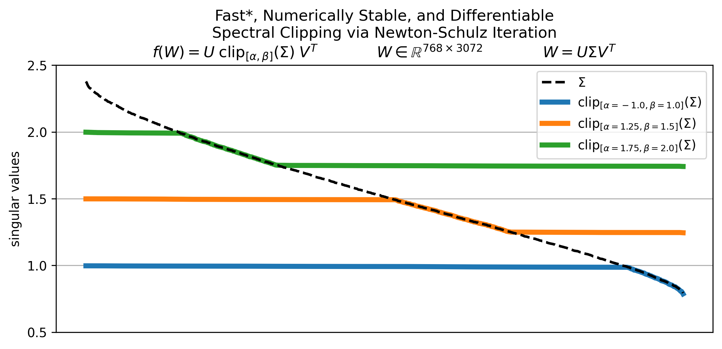
Definition 1 (Spectral Clipping). Let $W \in \mathbb{R}^{m \times n}$ and $W = U \Sigma V^T$ be its singular value decomposition where $\Sigma = (\sigma_1, \ldots, \sigma_{min(m,n)})$ are the singular values of $W$. Then we define Spectral Clipping as the following matrix function, $$\texttt{spectral\_clip}(W; \sigma_{max}) = U \texttt{clip}_{[-\sigma_{max}, \sigma_{max}]}(\Sigma) V^T$$ where $\sigma_{max} \in (0, \infty)$ is some hyperparameter that controls the spectral norm of the resulting matrix and $\texttt{clip}_{[\sigma_{min}, \sigma_{max}]}: \mathbb{R} \to \mathbb{R}$ is applied element-wise,

$$\texttt{clip}_{[\sigma_{min}, \sigma_{max}]}(x) = \begin{cases} \sigma_{min} & \texttt{if } x < \sigma_{min} \\ x & \texttt{if } \sigma_{min} \leq x \leq \sigma_{max} \\ \sigma_{max} & \texttt{if } \sigma_{max} < x \end{cases}$$

Note that we chose the $\texttt{clip}$ function above to be odd and symmetric because this allows us to use optimization tricks on computing matrix functions that only work on such functions. We will discuss more about this in the next sections.

Towards hardware-architecture-optimizer codesign

In deep learning, we not only have to be mindful of architecture-optimizer codesign but also hardware-software codesign. That is, architectural and optimizer choices and how we implement them have to be hardware-aware so that we can squeeze as much performance as we can from our GPUs/TPUs.

For example, the naive way to compute Spectral Clipping is to directly compute the SVD, clip the singular values we get from it, then reconstruct the matrix using the clipped singular values. A JAX implementation would look like this:

def naive_spectral_clip(W: jax.Array, sigma_max: float=1.):
    U, S, Vt = jnp.linalg.svd(W, full_matrices=False)
    S_clipped = jnp.clip(S, min=-sigma_max, max=sigma_max)
    return U @ jnp.diag(S_clipped) @ Vt

W = jax.random.normal(key, (m, n)) / 35.
W_clipped = naive_spectral_clip(W, sigma_max=1.)

However, this is not recommended because computing the SVD directly (1) does not take advantage of the GPUs’ tensor cores and (2) requires higher numerical precision, typically 32-bit float types. These not only slow things down but also increase precious memory usage, making it hard to scale to larger models.

Ideally, we want to only use operations that (1) have fast implementations on GPUs/TPUs and (2) are stable under lower numerical precision, e.g., 16-bit, 8-bit, even 4-bit float types. So, elementwise operations like matrix addition and scalar multiplication, matrix multiplication, matrix-vector products, among others are preferred, but not operations like matrix inversions or SVD decomposition, etc. With the proper coefficients, (semi-)orthogonalization via Newton-Schulz iteration for computing the matrix sign function has also been shown to be fast and numerically stable under lower precision (Jordan et al., 2024), thus we can use that here.

Finding a suitable surrogate function for $\texttt{clip}$

This is the fun part.

So, how do we compute spectral clipping while only using simple, but fast & numerically stable operations? First, let’s list the operations we can actually use and consider how they act on the matrix itself and its singular values. There are more operations we can use that aren’t listed here, but these would suffice for our problem.

Let’s reconstruct the $\mathbb{R} \to \mathbb{R}$ clipping on the singular values with these elementary functions first, then let’s use it to construct the matrix form. Here we take advantage of the following identities: $$\begin{align} |x| &= x \cdot \texttt{sign}(x) \\ \texttt{clip}_{[-1, 1]}(x) &= \frac{|1+x| - |1-x|}{2} \\ \texttt{clip}_{[\sigma_{min}, \sigma_{max}]}(x) &= \sigma_{max} \cdot \texttt{clip}_{[-1, 1]}(x / \sigma_{max}) \end{align}$$ These can easily be verified via elementary algebra. If you’re not convinced, see the figure below: Combining Equations (1) and (2), we get, $$\begin{equation}\texttt{clip}_{[-1, 1]}(x) = \frac{(1+x) \texttt{sign}(1+x) - (1-x) \texttt{sign}(1-x)}{2}\end{equation}$$

Lifting to matrix form

Naively lifting Equation (4) above to matrix form as in the following does not work:

$$\begin{equation}\frac{(1+W) \texttt{msign}(I+W) - (I-W) \texttt{msign}(1-W)}{2}\end{equation}$$

Why? Because $\texttt{msign}$ is only “aware” of the singular values of $I \pm W$, not $W$ itself. And so this matrix function does not properly “act” on the singular values of $W$ as we want it to.

However, recall that we constructed $\texttt{clip}$ to be an odd function. This allows us to Higham’s anti-block-diagonal trick (Higham, 2008) to lift the scalar function to matrix form.

Theorem 2 (Higham’s Anti-Block-Diagonal Trick). Let $g: \mathbb{R} \to \mathbb{R}$ be an odd analytic scalar function, $W \in \mathbb{R}^{m \times n}$, and construct the block matrix $S \in \mathbb{R}^{(m+n) \times (m+n)}$ as, $$S := \begin{bmatrix} 0 & W \\ W^T & 0 \end{bmatrix}$$ and let $g(S)$ as the primary matrix function defined from the scalar function $g$. Then, $$g(S) = \begin{bmatrix} 0 & g(W) \\ g(W^T) & 0 \end{bmatrix}$$ and hence, $$g(W) = [g(S)]_{12}$$

Setting $g = \texttt{clip}_{[-1, 1]}$ and applying Theorem 2, we can now properly construct $\texttt{spectral\_clip}(\cdot; 1)$ as follows: $$\begin{equation}\texttt{spectral\_clip}(W; 1) = \left[ \frac{(1+S) \texttt{msign}(I+S) - (I-S) \texttt{msign}(1-S)}{2} \right]_{12}\end{equation}$$ and following Equation (3), we can generalize this to any $\sigma_{max} > 0$ as follows, $$\begin{equation}\texttt{spectral\_clip}(W; \sigma_{max}) = \sigma_{max} \cdot \texttt{spectral\_clip}(W / \sigma_{max}; 1) \end{equation}$$

The following code implements this in JAX,

def _spectral_clip(W: jax.Array):
    m, n = W.shape
    I = jnp.eye(m + n)
    S = jnp.block([[jnp.zeros((m, m)), W], [W.T, jnp.zeros((n, n))]])
    gS = (1/2) * ((I + S) @ _orthogonalize(I + S) - (I - S) @ _orthogonalize(I - S))
    return gS[:m, m:]  # read off the top-right block

def spectral_clip(W: jax.Array, sigma_max: float=1.):
    return sigma_max * _spectral_clip(W / sigma_max)

where _orthogonalize_via_newton_schulz above implements Jordan’s (2024) Newton-Schulz iteration for computing the matrix sign function. Note however that we’re calling _orthogonalize_via_newton_schulz twice here, which is not ideal. Luckily, there’s a neat trick that allows us to compute it only once.

Optimizing the implementation via abstract algebra

First, notice that both $$I + S = \begin{bmatrix} I_m & W \\ W^T & I_n \end{bmatrix}\qquad I - S = \begin{bmatrix} I_m & -W \\ -W^T & I_n \end{bmatrix}$$ are block matrices of the form $$\begin{bmatrix} P & Q \\ Q^T & R \end{bmatrix}$$ where $P, R$ are symmetric matrices and $Q$ is an arbitrary matrix. It is a well-known result that such matrices form a linear sub-algebra $\mathcal{A}$, i.e., they are closed under addition, scalar multiplication, and matrix multiplication. This means that applying any polynomial function to these matrices will yield another matrix of the same form. And since we’re calculating the matrix sign function with Newton-Schulz iteration, which is a composition of polynomial functions, its result must also be of the same form.

Another neat property we can take advantage of is that flipping the signs of the anti-diagonal blocks gets preserved under application of matrix polynomials.

Proposition 3 (Parity w.r.t. $Q \to -Q$ when applying odd matrix polynomial $\texttt{p}(\cdot)$). Let $A \in \mathcal{A}$ such that, $$A = \begin{bmatrix} P & Q \\ Q^T & R \end{bmatrix}$$ and let, $$\begin{bmatrix} \widetilde{P} & \widetilde{Q} \\ \widetilde{Q}^T & \widetilde{R} \end{bmatrix} = \texttt{p}(A) = \texttt{p}\left(\begin{bmatrix} P & Q \\ Q^T & R \end{bmatrix}\right).$$ Then, $$\begin{bmatrix} \widetilde{P} & -\widetilde{Q} \\ -\widetilde{Q}^T & \widetilde{R} \end{bmatrix} = \texttt{p}\left(\begin{bmatrix} P & -Q \\ -Q^T & R \end{bmatrix}\right).$$

Crux of the proof: Flipping the sign of the anti-diagonal blocks gets preserved under addition, scalar multiplication, and matrix multiplication, $$\begin{bmatrix} 1 & -1 \\ -1 & 1 \end{bmatrix}\begin{bmatrix} 1 & -1 \\ -1 & 1 \end{bmatrix} \equiv \begin{bmatrix} 1 & -1 \\ -1 & 1 \end{bmatrix}$$

Thus we have, $$\begin{align} \begin{bmatrix} P^* & Q^* \\ Q^{*T} & R^{*} \end{bmatrix} &= \texttt{\_orthogonalize\_via\_newton\_schulz}(I + S) \\ \begin{bmatrix} P^{*} & -Q^{*} \\ -Q^{*T} & R^{*} \end{bmatrix} &= \texttt{\_orthogonalize\_via\_newton\_schulz}(I - S) \end{align}$$ for some $Q^{*} \in \mathbb{R}^{m \times n}$ and symmetric $P^{*} \in \mathbb{R}^{m \times m}$, $R^{*} \in \mathbb{R}^{n \times n}$. And combining these with Equation 6, we get,

$$\begin{align} \texttt{spectral\_clip}(W; 1) &= \left[\frac{\begin{bmatrix} I_m & W \\ W^T & I_n \end{bmatrix} \begin{bmatrix} P^{*} & Q^{*} \\ Q^{*T} & R^{*} \end{bmatrix} - \begin{bmatrix} I_m & -W \\ -W^T & I_n \end{bmatrix} \begin{bmatrix} P^{*} & -Q^{*} \\ -Q^{*T} & R^{*} \end{bmatrix}}{2}\right]_{12}\\ &= \left[\frac{\begin{bmatrix} P^{*} + WQ^{*T} & Q^{*} + WR^{*} \\ W^TP^{*}+Q^{*T} & W^TQ^{*} + R^{*} \end{bmatrix} - \begin{bmatrix} P^{*} + WQ^{*T} & -(Q^{*} + WR^{*}) \\ -(W^TP^{*}+Q^{*T}) & W^TQ^{*} + R^{*} \end{bmatrix}}{2}\right]_{12}\\ &= \begin{bmatrix} 0 & Q^{*} + WR^{*} \\ W^TP^{*}+Q^{*T} & 0 \end{bmatrix}_{12} \\ \texttt{spectral\_clip}(W; 1) &= Q^{*} + WR^{*} \\ \texttt{spectral\_clip}(W; \sigma_{max}) &= \sigma_{max} \cdot Q^{*} + WR^{*} \end{align}$$

This means that we only need to call _orthogonalize_via_newton_schulz once, and simply read off the blocks to compute the final result, leading to massive speedups. Also note that the diagonal blocks in Equation (12) are zero, which is what we expect from Theorem 2.

In JAX, this looks like the following:

def _spectral_clip(W: jax.Array):
    m, n = W.shape
    H = jnp.block([[jnp.eye(m), W], [W.T, jnp.eye(n)]])
    OH = _orthogonalize_via_newton_schulz(H)
    Q, R = OH[:m, m:], OH[m:, m:]
    return Q + W @ R

def spectral_clip(W: jax.Array, sigma_max: float=1.):
    return sigma_max * _spectral_clip(W / sigma_max, 1)

And a codegolf version would be,

def spectral_clip_minimal(W: jax.Array, sigma_max: float=1., ortho_dtype=jnp.float32):
    OH = _orthogonalize(jnp.block([[jnp.eye(W.shape[0]), W / sigma_max], [W.T / sigma_max, jnp.eye(W.shape[1])]]).astype(ortho_dtype)).astype(W.dtype)
    return sigma_max*OH[:W.shape[0], W.shape[0]:] + W @ OH[W.shape[0]:, W.shape[0]:]

Taking advantage of symmetry [Under Construction]

This section is still under construction. The crux is that we don’t actually need to materialize the entire $(m + n) \times (m + n)$ block matrix $S$ in memory and then do Newton-Schulz on it. Instead, we can maintain only the current $P$, $Q$, and $R$ blocks in memory, and handle matrix multiplications with extra care.

Experimental results [Under Construction]

This section is also still under construction.

Here

[NanoGPT Speedrun results will be added here]

References

1. Keller Jordan, Yuchen Jin, Vlado Boza, Jiacheng You, Franz Cesista, Laker Newhouse, and Jeremy Bernstein (2024). Muon: An optimizer for hidden layers in neural networks. Available at: https://kellerjordan.github.io/posts/muon/

References

- Greg Yang, James B. Simon, Jeremy Bernstein (2024). A Spectral Condition for Feature Learning. URL https://arxiv.org/abs/2310.17813
- Tim Large, Yang Liu, Minyoung Huh, Hyojin Bahng, Phillip Isola, Jeremy Bernstein (2024). Scalable Optimization in the Modular Norm. URL https://arxiv.org/abs/2405.14813
- Songlin Yang, Bailin Wang, Yu Zhang, Yikang Shen, and Yoon Kim (2025). Parallelizing Linear Transformers with the Delta Rule over Sequence Length. URL https://arxiv.org/abs/2406.06484
- Riccardo Grazzi, Julien Siems, Jörg K.H. Franke, Arber Zela, Frank Hutter, Massimiliano Pontil (2025). Unlocking State-Tracking in Linear RNNs Through Negative Eigenvalues. URL https://arxiv.org/abs/2411.12537
- Ali Behrouz, Zeman Li, Praneeth Kacham, Majid Daliri, Yuan Deng, Peilin Zhong, Meisam Razaviyayn, Vahab Mirrokni (2025). ATLAS: Learning to Optimally Memorize the Context at Test Time. URL https://arxiv.org/abs/2505.23735