Steepest Descent on Finsler-Structured (Matrix) Manifolds

If you find this post useful, please consider supporting my work by sponsoring me on GitHub:

1. Introduction

In this blog post, we shall consider the problem of steepest descent on Finsler-structured (matrix) manifolds. This problem naturally arises in deep learning optimization because we want model training to be fast and robust. That is, we want our weight updates to maximally change activations (or outputs) while keeping both activations and weights stable.

As discussed in prior blog posts and our latest paper, we can achieve this by properly considering the geometry in which to ‘place’ our weights in. This then begs the questions,

1. Which geometry should we ‘place’ our weights in? And,
2. How do we perform optimization in this geometry?

For (1), note that we have two degrees of freedom here: the choice of the underlying manifold and the choice of metric or norm to equip to the tangent spaces of the manifold. The latter makes (2) tricky because the manifold we end up with could not only be non-Euclidean but even non-Riemannian–and work on non-Riemannian optimization is scarce to almost non-existent.

While it might seem that we’re just inventing a difficult problem for bored mathematicians to solve, we will show in the next sections that we can motivate such problems with simple arguments and even lead to 1.5x to 2x speedup in large-scale LLM training.

This blog post generalizes work by Jeremy Bernstein and Jianlin Su on ‘Stiefel Muon’ to optimization on Finsler-structured (matrix) manifolds.

2. Case studies

2.1. Case study #1: Muon

2.2. Case study #2: Steepest descent on Spectral Finsler-structured ball around the origin

2.3. Case study #3: Steepest descent on Spectral Finsler-structured Stiefel manifold

The problem Jeremy, Jianlin, and I have been trying to solve then is this:

Given the current weight $W \in \texttt{St}(m, n) = \{ W \in \mathbb{R}^{m \times n} : W^T W = I_n \}$ and a “raw gradient” we get via e.g. backpropagation $G \in \mathbb{R}^{m \times n}$, we want to find the optimal update $A^*$ such that, $$\begin{equation} A^* = \arg\min_{A \in \mathbb{R}^{m \times n}} \langle G, A \rangle \quad \text{ s.t. } \quad \| A \|_{2 \to 2} \leq 1,\quad A \in T_{W}\texttt{St}(m, n) \end{equation}$$

Inspired by a partial solution by Jianlin (which did not yet work at the time), I proposed heuristic solutions here. Jianlin then solved the problem via a fixed-point iteration method. Finally, Jeremy proposed a more general solution via the dual ascent algorithm. Cédric Simal also independently proposed studying the dual problem to me and Jeremy.

3. General solution via block-wise Primal-Dual Hybrid Gradient (PDHG) algorithm

3.1. Problem statement

Let $\mathcal{M}$ be a (matrix) manifold and $\| \cdot \|$ be a Finsler norm defined on the tangent spaces of $\mathcal{M}$, both chosen a priori. We want to solve the problem,

Given the current weight $W \in \mathcal{M}$ and a “raw gradient” or differential we get via e.g. backpropagation $G \in T_{W}^*\mathcal{M} \subseteq \mathbb{R}^{m \times n}$, we want to find the optimal update $A^* \in T_{W}\mathcal{M} \subseteq \mathbb{R}^{m \times n}$ such that, $$\begin{equation} A^* = \arg\min_{A \in \mathbb{R}^{m \times n}} \langle G, A \rangle \quad \text{ s.t. } \quad \| A \|_{W} \leq \eta,\quad A \in T_{W}\mathcal{M} \end{equation}$$ where $\eta > 0$ is the learning rate parameter.

The $\langle \cdot, \cdot \rangle: T^*_{W}\mathcal{M} \times T_{W}\mathcal{M} \to \mathbb{R}$ operator above is not an inner product, but the canonical pairing between the cotangent and tangent spaces. It holds no geometric meaning by itself. But in the standard basis of $R^{m \times n}$, it coincidentally behaves like the Frobenius/Euclidean inner product. More intuitively, we can think of $\langle G, A \rangle$ as the directional derivative of the loss function in the direction of $A$. And we want to find the direction $A^*$ that maximally decreases the loss function while satisfying the constraints.

3.2. Convex optimization approach

First, notice that the feasible sets for the constraints on $A$ above are convex, regardless of where we currently are in the manifold. And so we can frame this problem squarely as a convex optimization problem.

Note: an intuitive, but incorrect approach is to simply project $G$ onto the (convex) intersection. First, this projection often does not have a closed-form solution. And second, it is suboptimal. Counterexample: suppose that $A=G$ is already in the intersection and $\langle G, A \rangle < 0$, but $\| A \|_{W} = 0.5\eta$. Then $2A$ must also be in the intersection, but $\langle G, 2A \rangle < \langle G, A \rangle$. Hence, naive projection onto the intersection is suboptimal.

There are many ways to solve this problem such as Alternating Direction Method of Multipliers (ADMM), Douglas-Rachford, and etc. In this blog post, we will focus on the Primal-Dual Hybrid Gradient (PDHG) method.

First, replace the constraints with indicator functions, $$\begin{equation} A^* = \arg\min_{A \in \mathbb{R}^{m \times n}} \left\{ \langle G, A \rangle + \mathcal{i}_{\| \cdot \|_{W} \leq \eta}(A) + \mathcal{i}_{T_{W}\mathcal{M}}(A) \right\} \end{equation}$$ where, $$ \mathcal{i}_{\| \cdot \|_{W} \leq \eta}(A) = \begin{cases} 0 &\text{ if } \| A \|_{W} \leq \eta \\ \infty &\text{ otherwise} \end{cases} \qquad \text{ and } \qquad \mathcal{i}_{T_{W}\mathcal{M}}(A) = \begin{cases} 0 &\text{ if } A \in T_{W}\mathcal{M} \\ \infty &\text{ otherwise} \end{cases} $$

Equivalently, $$\begin{equation} A^* = \arg\min_{A \in \mathbb{R}^{m \times n}} \left\{ f_{\eta}(A) + g(A) \right\} \end{equation}$$ where $f_{\eta}(\cdot) := \mathcal{i}_{\| \cdot \|_{W} \leq \eta}(\cdot)$ and $g(\cdot) := \mathcal{i}_{T_{W}\mathcal{M}}(\cdot) + \langle G, \cdot \rangle$. Note that we can move the $\langle G, \cdot \rangle$ term to $f$ instead, but as we will see later, the proximal operator for $g$ is simpler so we keep it there for improved numerical stability.

We can then split Equation (4) into two subproblems by ‘copying’ $A$, $$\begin{equation} A^* = \left[\arg\min_{A,B \in \mathbb{R}^{m \times n}} \{f_{\eta}(A) + g(B)\} \quad \text{ s.t. } \quad A - B = 0\right]_{A} \end{equation}$$ This effectively blows up our solution search space, but one can easily prove that the optimal solution to the problem above also solves our original problem!

3.3. Recasting as a primal-dual problem

Define, $$ \begin{align*} X &:= \begin{bmatrix} A \\ B \end{bmatrix}\\ L &:= \begin{bmatrix} I & -I \end{bmatrix} \\ \mathcal{F}_{\eta}(X) &:= f_{\eta}(A) + g(B) \\ \mathcal{G}(Y) &:= \mathcal{i}_{\{0\}}(Y) = \begin{cases} 0 &\text{ if } Y = 0 \\ \infty &\text{ otherwise} \end{cases} \end{align*} $$ where $X \in \mathcal{X} = \mathbb{R}^{2m \times n}$, $Y \in \mathcal{Y} = \mathbb{R}^{m \times n}$, $L: \mathcal{X} \to \mathcal{Y}$ is a linear operator, $\mathcal{F}_{\eta}: \mathcal{X} \to \mathbb{R}$, and $\mathcal{G}: \mathcal{Y} \to \mathbb{R}$.

Then Equation (5) can be rewritten to, $$\begin{align} A^* &= \left[ \arg\min_{X \in \mathcal{X}} \{\mathcal{F}_{\eta}(X) + \mathcal{G}(LX)\} \right]_{1} \end{align}$$

Fenchel duality then yields the saddle problem, $$\begin{align} \min_{X \in \mathcal{X}} \max_{Y \in \mathcal{Y}} \mathcal{L}(X,Y) &:= \mathcal{F}_{\eta}(X) + \langle LX, Y \rangle - \mathcal{G}^*(Y) \nonumber \\ &\ = \mathcal{F}_{\eta}(X) + \langle LX, Y \rangle \end{align}$$ since $\mathcal{G}^*(Y) = \sup_{Z \in \mathcal{Y}} \{ \langle Y, Z \rangle - \underbrace{\mathcal{G}(Z)}_{=\infty \text{ if } Z \neq 0} \} = \langle Y, 0 \rangle + \mathcal{G}(0) = 0$ for all $Y \in \mathcal{Y}$.

3.4. Block-wise Primal-Dual Hybrid Gradient

Following ODL’s page on PDHG, we choose $\tau_A, \tau_B, \sigma > 0$, $\theta \in [0,1]$, and initialize $X_0 \in \mathcal{X}$, $Y_0 \in \mathcal{Y}$, and $\widetilde{X}_0 = X_0$. We then iterate, $$\begin{align} Y_{k+1} &= \texttt{prox}_{\sigma \mathcal{G}^*} (Y_{k} + \sigma L \widetilde{X}_{k}) \\ X_{k+1} &= \texttt{prox}_{\tau \mathcal{F}_{\eta}} (X_{k} - \tau L^T Y_{k+1}) \\ \widetilde{X}_{k+1} &= X_{k+1} + \theta (X_{k+1} - X_{k}) \end{align}$$ where $\tau = \text{diag}(\tau_A I_m, \tau_B I_m)$ and $\texttt{prox}$ is the proximal operator.

To speed up convergence, we can also re-use the $X^*$ and $Y^*$ from the previous optimization step to initialize $X_0$ and $Y_0$. This is especially useful when e.g. using (nesterov) momentum on $G$, guaranteeing that the ‘input gradients’ do not vary too much.

3.4.1. Converting proximal operators to projections

For the $Y$-variable, $$\begin{align*} Y_{k+1} &= \texttt{prox}_{\sigma \mathcal{G}^*} (Y_{k} + \sigma L \widetilde{X}_{k}) \\ &= \arg\min_{Y \in \mathcal{Y}} \left\{ \sigma \cancel{\mathcal{G}^*(Y)} + \frac{1}{2} \| Y - (Y_{k} + \sigma L \widetilde{X}_{k}) \|_F^2 \right\} \\ &= Y_{k} + \sigma L \widetilde{X}_{k} \end{align*}$$

For the $X$-variable, $$\begin{align*} X_{k+1} &= \texttt{prox}_{\tau \mathcal{F}_{\eta}} (X_{k} - \tau L^T Y_{k+1}) \\ &= \arg\min_{X \in \mathcal{X}} \left\{ \tau \mathcal{F}_{\eta}(X) + \frac{1}{2} \| X - (X_{k} - \tau L^T Y_{k+1}) \|_F^2 \right\} \\ &= \arg\min_{X \in \mathcal{X}} \left\{ \tau_A f_{\eta}(A) + \tau_B g(B) + \frac{1}{2} \left\| \begin{bmatrix} A - (A_k - \tau_A Y_{k+1}) \\ B - (B_k + \tau_B Y_{k+1}) \end{bmatrix} \right\|_F^2 \right\} \\ &= \arg\min_{X \in \mathcal{X}} \{ \tau_A f_{\eta}(A) + \frac{1}{2} \left\| A - (A_k - \tau_A Y_{k+1}) \right\|_F^2 \\ &\qquad\qquad + \tau_B g(B) + \frac{1}{2} \left\| B - (B_k + \tau_B Y_{k+1}) \right\|_F^2 \} \\ \end{align*}$$

Note that we can optimize for $A$ and $B$ separately and thus get, $$\begin{align*} A_{k+1} &= \arg\min_{A \in \mathbb{R}^{m \times n}} \left\{ \tau_A f_{\eta}(A) + \frac{1}{2} \left\| A - (A_k - \tau_A Y_{k+1}) \right\|_F^2 \right\} \\ &= \arg\min_{\| A \|_{W} \leq \eta} \left\{ \frac{1}{2} \left\| A - (A_k - \tau_A Y_{k+1}) \right\|_F^2 \right\} \\ &= \texttt{proj}_{\| \cdot \|_{W} \leq \eta} (A_k - \tau_A Y_{k+1}) \\ \end{align*}$$ where $\texttt{proj}_{\| \cdot \|_{W} \leq \eta}$ is the projection onto the ${\eta}$-norm ball. Likewise, $$\begin{align*} B_{k+1} &= \arg\min_{B \in \mathbb{R}^{m \times n}} \left\{ \tau_B g(B) + \frac{1}{2} \left\| B - (B_k + \tau_B Y_{k+1}) \right\|_F^2 \right\} \\ &= \arg\min_{B \in T_W\mathcal{M}} \left\{ \tau_B \langle G, B \rangle + \frac{1}{2} \left\| B - (B_k + \tau_B Y_{k+1}) \right\|_F^2 \right\} \\ &= \arg\min_{B \in T_W\mathcal{M}} \left\{ \tau_B \langle G, B \rangle + \frac{1}{2} \| B \|_F^2 - \langle B, B_k + \tau_B Y_{k+1} \rangle + \frac{1}{2} \| B_k + \tau_B Y_{k+1} \|_F^2 \right\} \\ &= \arg\min_{B \in T_W\mathcal{M}} \left\{ \frac{1}{2} \| B \|_F^2 - \langle B, B_k + \tau_B Y_{k+1} - \tau_B G \rangle + \text{ constant} \right\} \\ &= \arg\min_{B \in T_W\mathcal{M}} \left\{ \frac{1}{2} \| B - (B_k + \tau_B Y_{k+1} - \tau_B G) \|_F^2 + \text{ constant} \right\} \\ &= \texttt{proj}_{T_W\mathcal{M}} (B_k + \tau_B Y_{k+1} - \tau_B G) \end{align*}$$ Thus, $$ \begin{equation} X_{k+1} = \begin{bmatrix} \texttt{proj}_{\| \cdot \|_{W} \leq \eta} (A_k - \tau_A Y_{k+1}) \\ \texttt{proj}_{T_W\mathcal{M}} (B_k + \tau_B Y_{k+1} - \tau_B G) \end{bmatrix} \end{equation} $$

3.4.2. Block-wise PDHG algorithm for the steepest descent on Finsler manifolds problem

Taking everything together, our iteration becomes,

$$\begin{align} Y_{k+1} &= Y_{k} + \sigma (\widetilde{A}_{k} - \widetilde{B}_{k}) \\ A_{k+1} &= \texttt{proj}_{\| \cdot \|_{W} \leq \eta} (A_k - \tau_A Y_{k+1}) \\ B_{k+1} &= \texttt{proj}_{T_W\mathcal{M}} (B_k + \tau_B Y_{k+1} - \tau_B G) \\ \widetilde{A}_{k+1} &= A_{k+1} + \theta (A_{k+1} - A_{k}) \\ \widetilde{B}_{k+1} &= B_{k+1} + \theta (B_{k+1} - B_{k}) \end{align}$$

Note that if we had moved the $\langle G, \cdot \rangle$ to the $f$ term in Equation (4), then our iteration for $A$ and $B$ would instead be,

$$\begin{align} A_{k+1} &= \texttt{proj}_{\| \cdot \|_{W} \leq \eta} (A_k - \tau_A Y_{k+1} - \tau_A G) \\ B_{k+1} &= \texttt{proj}_{T_W\mathcal{M}} (B_k + \tau_B Y_{k+1}) \\ \end{align}$$ In theory, both iterations should converge to the same solution. But in practice, the former tends to be more numerically stable.

4. Alternative solution to Stiefel Muon via Primal-Dual Hybrid Gradient algorithm

One way to prevent neural network training from blowing up is to constrain the linear layers of our neural network to be $L$-Lipschitz under the $\texttt{RMS}$ norm (ideally with $L=1$ so that the Lipschitzness of the model is depth-independent). Another thing we would want to do is to control the update sizes. And in this setting, it is natural to upper bound the $\texttt{RMS}\to\texttt{RMS}$ operator norm of the weight updates by $\eta > 0$, the learning rate parameter.

We discussed multiple ways to do this in our paper Training Transformers with Enforced Lipschitz Bounds. The crux is to upper bound the singular values of the weights by $\sqrt{\frac{m}{n}}$ and to use the Muon optimizer for weight updates. But here, suppose we want the singular values of the weights to be exactly $\sqrt{\frac{m}{n}}$ instead. Then it is natural to “place” the weights on the scaled Stiefel manifold, $\texttt{St}(m, n, s) = \{ W \in \mathbb{R}^{m \times n} : W^T W = s^2 I_n \}$ where $s = \sqrt{\frac{m}{n}}$ and perform steepest descent there. How then would the update rule look like?

4.1. Required projections

As we discussed above and in Heuristic Solutions for Steepest Descent on the Stiefel Manifold, we need the following projections:

1. Projection onto the (scaled) Stiefel manifold, $\texttt{proj}_{\widetilde{\texttt{St}}(m, n, \sqrt{m/n})}: \mathbb{R}^{m \times n} \to \widetilde{\texttt{St}}(m, n, \sqrt{m/n})$, as the retraction map.
2. Projection onto the tangent space at $W \in \widetilde{\texttt{St}}(m, n, \sqrt{m/n})$, $\texttt{proj}_{T_{W}\widetilde{\texttt{St}}(m, n, \sqrt{m/n})}: \mathbb{R}^{m \times n} \to T_W\widetilde{\texttt{St}}(m, n, \sqrt{m/n})$. And;
3. Projection onto the $\texttt{RMS}\to\texttt{RMS}$ norm ball, $\texttt{proj}_{\| \cdot \|_{\texttt{RMS} \to \texttt{RMS}} \leq \eta}: \mathbb{R}^{m \times n} \to \{ A \in \mathbb{R}^{m \times n} : \| A \|_{\texttt{RMS} \to \texttt{RMS}} \leq \eta \}$.

For (1), we can use the GPU-friendly method to compute the $\texttt{msign}(X)$ function via Newton-Schulz iteration as in the Muon optimizer, $$\texttt{proj}_{\widetilde{\texttt{St}}(m, n, \sqrt{m/n})}(X) = \sqrt{\frac{m}{n}} \texttt{msign}(X).$$

For (2), we can use the projection map discussed in Theorem 2 in Heuristic Solutions for Steepest Descent on the Stiefel Manifold, $$\texttt{proj}_{T_{W}\texttt{St}(m, n)}(X) = X - {W} \text{sym}({W}^T X).$$ More generally, for the scaled Stiefel manifold, we have, $$\texttt{proj}_{T_{W}\widetilde{\texttt{St}}(m, n, s)}(V) = V - {W} \text{sym}({W}^T V) / s^2.$$

For (3), note that $\|\cdot \|_{\texttt{RMS}\to\texttt{RMS}} = \sqrt{\frac{n}{m}} \|\cdot \|_{2 \to 2}$. Thus, $$ \begin{aligned} \texttt{proj}_{\| \cdot \|_{\texttt{RMS} \to \texttt{RMS}} \leq \eta} &= \texttt{proj}_{\| \cdot \|_{2 \to 2} \leq \sqrt{\frac{m}{n}}\eta} \\ &= \texttt{spectral\_hardcap}_{\sqrt{\frac{m}{n}}\eta} \end{aligned} $$ where $\texttt{spectral\_hardcap}$ is the GPU/TPU-friendly Spectral Hardcap function discussed in Fast, Numerically Stable, and Auto-Differentiable Spectral Clipping via Newton-Schulz Iteration and in our latest paper,

def spectral_hardcap(X: jax.Array, eta: float=1.):
    def _spectral_hardcap_util(X: jax.Array):
        if transpose := X.shape[0] > X.shape[1]:
            X = X.T
        result = (1/2) * ((OX := orthogonalize(X)) + X - orthogonalize(jnp.eye(X.shape[0]) - OX @ X.T) @ (OX - X))
        if transpose:
            result = result.T
        return result
    return eta * _spectral_hardcap_util(X / eta)

But if $G$ small, we may be able to find larger update directions by scaling the input to $\texttt{spectral\_hardcap}$ by some large constant $\kappa \geq 1$ yielding, $$\lim_{\kappa \to \infty} \texttt{spectral\_hardcap}_{\sqrt{\frac{m}{n}}\eta}(\kappa X) = \sqrt{\frac{m}{n}}\eta \cdot \texttt{msign}(X).$$

4.2. Full implementation with adaptive step sizes

def pdhg(
    W: jax.Array,
    G: jax.Array,
    proj_norm_ball: Callable[[jax.Array], jax.Array],
    proj_tangent_space: Callable[[jax.Array, jax.Array], jax.Array],
    *,
    tau_A=1.0, tau_B=1.0, sigma=0.49, gamma=1.,
    max_iters=200, tol=1e-6,
    A0=None, B0=None, Y0=None
) -> jax.Array:
    m, n = W.shape
    A = jnp.zeros((m, n), W.dtype) if A0 is None else A0
    B = jnp.zeros((m, n), W.dtype) if B0 is None else B0
    Y = jnp.zeros((m, n), W.dtype) if Y0 is None else Y0
    A_bar, B_bar = A, B

    def cond(state):
        _, _, _, _, _, k, res, *_= state
        return jnp.logical_and(k < max_iters, res > tol)

    def body(state):
        A, B, Y, A_bar, B_bar, k, _, tau_A, tau_B, sigma = state

        # Dual ascent
        Y_new = Y + sigma * (A_bar - B_bar)

        # Primal descent (A & B updates)
        A_new = proj_norm_ball(A - tau_A * Y_new)
        B_new = proj_tangent_space(W, B + tau_B * Y_new - tau_B * G)

        # A_new = proj_norm_ball(A - tau_A * Y_new - tau_A * G)
        # B_new = proj_tangent_space(W, B + tau_B * Y_new)

        # update step-sizes
        tau = 0.5 * (tau_A + tau_B)
        theta = 1 / jnp.sqrt(1 + 2 * gamma * tau)
        tau_A = theta * tau_A
        tau_B = theta * tau_B
        sigma = sigma / theta

        # Extrapolation
        A_bar_new = A_new + theta * (A_new - A)
        B_bar_new = B_new + theta * (B_new - B)

        res = jnp.linalg.norm(A_new - B_new)

        return (A_new, B_new, Y_new, A_bar_new, B_bar_new, k+1, res, tau_A, tau_B, sigma)

    init = (A, B, Y, A_bar, B_bar, 0, jnp.inf, tau_A, tau_B, sigma)
    A, B, Y, *_ = jax.lax.while_loop(cond, body, init)
    return A

def pdhg_stiefel_spectral(
    W: jax.Array, G: jax.Array, target_norm=1., *,
    tau_A=1., tau_B=1., sigma=0.49, gamma=1.,
    max_iters=200, tol=1e-6,
    A0=None, B0=None, Y0=None
) -> jax.Array:
    return pdhg(
        W, G,
        # proj_norm_ball=lambda X: spectral_hardcap(X, target_norm),
        proj_norm_ball=lambda X: target_norm * orthogonalize(X),
        proj_tangent_space=project_to_stiefel_tangent_space,
        tau_A=tau_A, tau_B=tau_B, sigma=sigma, gamma=gamma,
        max_iters=max_iters, tol=tol,
        A0=A0, B0=B0, Y0=Y0
    )

To speed up convergence, we can warm-start the iteration by initializing $A_0$ and $B_0$ with a decent guess. Here are a few options:

1. $A_0 = B_0 = -G$.
2. $A_0 = B_0 = \left(\texttt{proj}_{\| \cdot \|_{\texttt{RMS} \to \texttt{RMS}} \leq \eta} \circ \texttt{proj}_{T_{W}\widetilde{\texttt{St}}(m, n, \sqrt{m/n})} \right)(-G)$, which is already optimal for the square case. And;
3. $A_0 = B_0 = \left(\texttt{proj}_{\| \cdot \|_{\texttt{RMS} \to \texttt{RMS}} \leq \eta} \circ \texttt{proj}_{T_{W}\widetilde{\texttt{St}}(m, n, \sqrt{m/n})} \right)^K (-G)$, the alternating projections method discussed in Heuristic Solutions for Steepest Descent on the Stiefel Manifold.

In the succeeding training steps, we can then initialize $A_0$ and $B_0$ with the optimal $A^*$ from the previous step.

4.3. Experimental results

Here I’ve plotted the alignment <-> off-tangency frontier for the different methods for computing the optimal descent direction in Stiefel Muon proposed by myself, Jeremy, and Jianlin.

4.3.1. Case 1: Full-rank $G$

For the case where $G$ is full-rank, we see that the Alternating Projections method I proposed in Heuristic Solutions for Steepest Descent on the Stiefel Manifold does quite well despite being provably suboptimal in some cases. The PDHG method closes the gap as we increase the number of iterations, but it and the other methods perform roughly similarly.

4.3.2. Case 2: $G$ is rank-deficient

For the rank-deficient case, we see that the Alternating Projections is now obviously suboptimal. Jianlin’s and Jeremy’s methods perform similarly. And finally, the PDHG method not only results in updates $A$ that are more aligned with the ‘raw gradient’ $G$, but are least off-tangent as well.

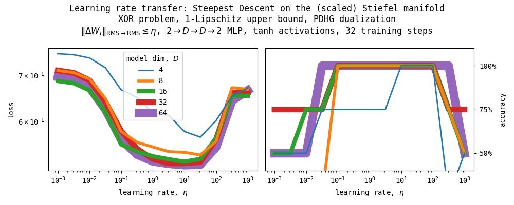
4.3.3. Learning rate transfer, XOR problem

As a minimal example for learning rate transfer, we train a $1$-Lipschitz, $2 \to D \to D \to 2$ MLP on the XOR problem for 32 training steps via the Modula library. We constrain the weights of each layer to be in the (scaled) Stiefel manifold. We use $\texttt{msign}_{\sqrt{m/n}}: \mathbb{R}^{m \times n} \to \widetilde{\texttt{St}}\left(m, n, \sqrt{m/n}\right)$ as the projection map onto the scaled Stiefel manifold (with scale $\sqrt{m/n}$) and PDHG, $\texttt{pdhg}\left(\cdot, \cdot, \texttt{msign}_{\eta}, \texttt{proj}_{T_{W_{t}}\widetilde{\texttt{St}}\left(m, n, \sqrt{m/n}\right)}\right): \mathbb{R}^{m \times n} \to T_{W_t} \widetilde{\texttt{St}}\left(m, n, \sqrt{m/n}\right)$, as the dualizer. As can be seen in the Figure above, the optimal learning rates do transfer under our parametrization.

5. Generalization to arbitrary number of constraints on the update

Our solution above generalizes to arbitrary number of constraints on $A$ so long as the feasible set for each constraint is convex. We then only need to find the metric projection onto each feasible set.

For example, suppose we add another constraint $A \in S$ in Equation (2) above where $S$ is a convex set and $\texttt{proj}_{S}(\cdot)$ is the (metric) projection onto $S$. Then our Equation (5) becomes, $$\begin{equation} A^* = -\left[\arg\min_{A,B,C \in \mathbb{R}^{m \times n}} \{f(A) + g(B) + h(C)\} \quad \text{ s.t. } \quad A - B = A - C = 0\right]_{A} \end{equation}$$ where, $$ h(C) := \mathcal{i}_{S}(C) = \begin{cases} 0 &\text{ if } C \in S \\ \infty &\text{ otherwise} \end{cases} $$

We then define, $$ \begin{align*} X &:= \begin{bmatrix} A \\ B \\ C \end{bmatrix}\\ L &:= \begin{bmatrix} I & -I & \\ I & & -I \end{bmatrix} \\ \mathcal{F}(X) &:= f(A) + g(B) + h(C) \\ \end{align*} $$ and the rest then follows and Equation (11) becomes, $$ \begin{equation} X_{k+1} = \begin{bmatrix} \texttt{proj}_{\| \cdot \|_{W} \leq \eta} (A_k - \tau_A [Y_{k+1}]_1 - \tau_A [Y_{k+1}]_2) \\ \texttt{proj}_{T_W\mathcal{M}} (B_k + \tau_B [Y_{k+1}]_1 - \tau_B G) \\ \texttt{proj}_{S} (C_k + \tau_C [Y_{k+1}]_2) \end{bmatrix} \end{equation} $$

Acknowledgements

Big thanks to Jeremy Bernstein, Cédric Simal, and Antonio Silveti-Falls for productive discussions on the topic! All remaining mistakes are mine.

How to cite

@misc{cesista2025steepestdescentfinsler,
  author = {Franz Louis Cesista},
  title = {{S}teepest {D}escent on {F}insler-Structured (Matrix) {M}anifolds},
  year = {2025},
  month = {August},
  day = {20},
  url = {https://leloykun.github.io/ponder/steepest-descent-finsler/},
}

If you find this post useful, please consider supporting my work by sponsoring me on GitHub:

References

1. Jeremy Bernstein (2025). Stiefel manifold. URL https://docs.modula.systems/algorithms/manifold/stiefel/
2. Jianlin Su (2025). Muon + Stiefel. URL https://kexue.fm/archives/11221
3. Laker Newhouse, R. Preston Hess, Franz Cesista, Andrii Zahorodnii, Jeremy Bernstein, Phillip Isola (2025). Training Transformers with Enforced Lipschitz Bounds. URL https://arxiv.org/abs/2507.13338
4. Jeremy Bernstein & Laker Newhouse (2024). Old optimizer, new norm: an anthology. URL https://arxiv.org/abs/2409.20325
5. Keller Jordan and Yuchen Jin and Vlado Boza and Jiacheng You and Franz Cesista and Laker Newhouse and Jeremy Bernstein (2024). Muon: An optimizer for hidden layers in neural networks. URL https://kellerjordan.github.io/posts/muon/
6. Greg Yang, James B. Simon, Jeremy Bernstein (2024). A Spectral Condition for Feature Learning. URL https://arxiv.org/abs/2310.17813
7. ODL (2020). Primal-Dual Hybrid Gradient Algorithm (PDHG). URL https://odlgroup.github.io/odl/math/solvers/nonsmooth/pdhg.html
8. Jeremy Bernstein (2025). The Modula Docs. URL https://docs.modula.systems/