1. Introduction
In this blog post, we shall consider the problem of steepest descent on Finsler-structured (matrix) geometries. This problem naturally arises in deep learning optimization because we want model training to be fast and robust. That is, we want our updates to maximally change weights and activations (or “features”) so that we can train larger models more quickly while also keeping activation, weight, and gradient norms within some reasonable bounds to guarantee that our expensive training runs would not randomly blow up halfway through.
$\blacksquare$ Let us start on robustness: as we discussed in Ponder: Training Transformers with Enforced Lipschitz Constants and Ponder: Rethinking Maximal Update Parametrization: Steepest Descent on the Spectral Ball, we can achieve our robustness goals by enforcing both layer-wise and global Lipschitz constraints on our models. Intuitively, Lipschitzness is the knob that controls how fast our features “grow” in the forward pass and how fast our gradients “grow” in the backward pass. Lower Lipschitzness then guarantees stabler training dynamics and flatter loss landscapes. But why do we want layer-wise Lipschitz constraints? That is because we can convert any possibly-highly-unstable $L$-Lipschitz model into a globally 1-Lipschitz model by scaling its final logits by $1/L$, and this does nothing to prevent intermediate activations and gradients from blowing up.
To enforce layer-wise Lipschitz constraints, we have to consider parameter-free and parametrized layers separately. In Ponder: Sensitivity and Sharpness of n-Simplicial Attention, we previously derived a parametrization of $n$-Simplicial Attention (Roy et al., 2025) that is 1-Lipschitz by construction, generalizing prior work by Large et al. (2024). And for parametrized layers, we can enforce Lipschitz constraints by bounding the induced operator norm (from the chosen feature norms) of the weight matrices (Newhouse et al., 2025). In this blog post, we shall focus on the latter.
A neat consequence of controlling the weight and update norms is that, by the norm equivalence theorem for finite dimensions, we also bound the size of our weight and update matrix entries. A low-enough bound allows us to shave off bits from our floating-point representations without overflowing or underflowing, enabling more aggressive quantization-aware training, basically “for free”, as we have demonstrated in Training Transformers with Enforced Lipschitz Constants.
$\blacksquare$ Now, let us consider our other goal: maximal updates for faster training. For this, we need to consider (1) how we measure the “size” of our updates and (2) how to make sure that our updates do not interfere with our weight control mechanisms. Combining these with our need to constrain the weights to some bounded set naturally leads us to the problem of optimization on some normed geometry. But which geometry and what norm?
In this blog post, we shall consider the general case where we constrain the weights to some manifold $\mathcal{M}$ whose points $W \in \mathcal{M}$ have tangent spaces $T_{W}\mathcal{M}$ equipped with some possibly point-dependent, non-Euclidean, or even non-Riemannian norm $\| \cdot \|_{W}$. Our method also works for cone geometries such as the positive semidefinite cone and the spectral band where boundary points could instead have tangent cones where $V \in T_{W}\mathcal{M}$ does not imply $-V \in T_{W}\mathcal{M}$.
Another neat consequence of doing steepest descent under the induced operator norm is that it enables learning rate transfer across model widths, given that the feature norms we induce the operator norms from also scale appropriately with model width (Pethick et al., 2025; Bernstein et al., 2024; Filatov et al., 2025). We will discuss this in more detail in Section 2.2.
This work expands on and generalizes prior work by Bernstein (2025), Keigwin, et al. (2025), Cesista (2025), and Su (2025) on ‘Manifold Muon’.
2. Preliminaries
2.1. (Decoupled) weight decay as weight constraint (and why it is suboptimal)

Weight decay already (implicitly) constraints weights to some bounded set. We discussed this in more detail in Appendix A2 of Ponder: Rethinking Maximal Update Parametrization: Steepest Descent on the Spectral Ball.
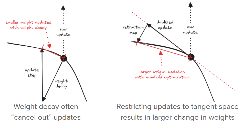
The crux is that the “backtracking” weight decay grows linearly with the weight norm, but the update sizes from our optimizers remain roughly constant. For example, with Muon, the update sizes are guaranteed to have spectral norm at most $\eta$, the learning rate; with Adam and variants such as SignSGD, it is the elementwise max-norm that is bounded by $\eta$. And so, if the weight is “too large”, backtracking dominates the update, and the weight norm shrinks; if the weight is “too small”, the update dominates backtracking, and the weight norm grows. At equilibrium, the backtracking and update sizes balance out, and the weight norm stabilizes. Thus, weight decay already helps enforce Lipschitz constraints to some extent.
But weight decay also often “interferes” with the updates. For example, when the gradients are aligned with the weights. And as we will show in Section 4, this interference results in smaller effective update sizes and slows down generalization. Hence why, in this blog post, we replace weight decay with proper manifold optimization in the weight space.
2.2. “Natural” feature and weight norms
As we mentioned in the introduction, we can enable learning rate transfer across model widths by choosing a feature norm that scales appropriately with model width (Pethick et al., 2025; Bernstein et al., 2024; Filatov et al., 2025). We argue that the “natural” feature norm is a norm that is preserved under concatenation. More precisely, for all $x \in \mathbb{R}^n$ and $y \in \mathbb{R}^m$, we want,
$$\begin{equation} \| x \| = \| y \| = c \implies \left\| \begin{bmatrix} x \\ y \end{bmatrix} \right\| = c, \end{equation}$$for $c \geq 0$. The $\texttt{RMS}$ norm, $\| \cdot \|_{\texttt{RMS}} = \frac{1}{\sqrt{n}} \| \cdot \|_F$, satisfies this criterium, and so it is a good candidate for the “natural” feature norm. This then induces the $\texttt{RMS}\to\texttt{RMS}$ norm,
$$\begin{equation} \| A \|_{\texttt{RMS}\to\texttt{RMS}} = \sup_{x \neq 0} \frac{\| Ax \|_{\texttt{RMS}}}{\| x \|_{\texttt{RMS}}} = \sup_{x \neq 0} \frac{\| Ax \|_{2} / \sqrt{m}}{\| x \|_{2} / \sqrt{n}} = \sqrt{\frac{n}{m}} \| A \|_{2 \to 2}, \end{equation}$$as a good candidate for the “natural” weight norm. Yang et al. (2024) also makes a similar argument.
2.3. Constrained first-order optimization on Finsler geometries
Let $f: \mathcal{M} \to \mathbb{R}$ be a differentiable and bounded-below objective function defined on our Finsler geometry of interest $\mathcal{M}$. That is, a constraint set $\mathcal{M} \subseteq \mathbb{R}^{m \times n}$ equipped with a (possibly point-dependent) norm $\|\cdot\|_{W_t}$ on each tangent set, $T_{W_t}\mathcal{M}$, at each point $W_t \in \mathcal{M}$. First-order optimization on such geometries goes as follows:
- Let $W_t \in \mathcal{M}$ be the ‘weight’ parameter at time step $t$. Compute the “raw gradient” $G_t = \nabla f(W_t)$ via e.g. backpropagation.
- Compute an ‘optimal’ descent direction $A^*_t \in T_{W_t} \mathcal{M}$ under the norm in the tangent set at $W_t$ constrained as, $$\begin{align} A^*_t &= \arg\min_{A \in \mathbb{R}^{m \times n}} f(W_t) + \langle G_t, A \rangle \quad \text{ s.t. } \quad \| A \|_{W_t} \leq \eta,\quad A \in T_{W_t}\mathcal{M} \nonumber \\ &= \arg\min_{A \in \mathbb{R}^{m \times n}} \langle G_t, A \rangle \quad \text{ s.t. } \quad \| A \|_{W_t} \leq \eta,\quad A \in T_{W_t}\mathcal{M}, \label{eq:optimaldescent} \end{align}$$ where $\eta > 0$ is the learning rate hyperparameter.
- Update the weight in the direction of $A^*_t$ and retract the result back to the manifold via a retraction map, $\texttt{retract}_{\mathcal{M}}: \mathbb{R}^{m \times n} \to \mathcal{M}$, $$W_{t+1} \leftarrow \texttt{retract}_{\mathcal{M}}(W_t + A^*_t).$$
Note that both constraints on $A$ in Equation $\eqref{eq:optimaldescent}$ are membership constraints to closed convex sets, and so it is simply a convex optimization problem.
$\blacksquare$ Special case: if $T_{W_t}\mathcal{M} = \mathbb{R}^{m \times n}$, then we can solve the problem via a Linear Minimization Oracle (LMO) (Pethick et al., 2025) for the chosen norm,
$$\begin{align} A^*_t &= \arg\min_{\| A \|_{W_t} \leq \eta} \langle G_t, A \rangle \nonumber \\ &= \eta \cdot \arg\min_{\| A \|_{W_t} \leq 1} \langle G_t, A \rangle \nonumber \\ &= \eta \cdot \text{LMO}_{\|\cdot\|_{W_t}}(G_t). \nonumber \end{align}$$Unfortunately, as we have discussed in Ponder: Heuristic Solutions for Steepest Descent on the Stiefel Manifold, LMOs typically do not preserve tangency for general $T_{W_t}\mathcal{M}$, requiring more complicated solutions to solve Equation $\eqref{eq:optimaldescent}$. We will discuss one such solution via dual ascent in the next section.
3. Steepest descent on Finsler geometries via dual ascent
3.1. General strategy
Our goal is to solve Equation $\eqref{eq:optimaldescent}$ for any choice of norm $\|\cdot\|_{W_t}$ and tangent set $T_{W_t}\mathcal{M}$. Let the latter be represented as,
$$\begin{equation} T_{W_t}\mathcal{M} = \{ A \in \mathbb{R}^{m \times n} \mid L_{W_t}(A) + b_{W_t} \in -K \} \label{eq:tangentset} \end{equation}$$for some (possibly point-dependent) linear map $L_{W_t}: \mathbb{R}^{m \times n} \to \mathcal{Y}$, constant offset $b_{W_t} \in \mathcal{Y}$ (often $b_{W_t} = 0$), and a closed convex cone $K \subseteq \mathcal{Y}$. Equality constraints can be represented by setting $K = \{0\}$. For example, for the Stiefel manifold, we have $L_{W}(A) = W^\top A + A^\top W$ and $K = \{0\}$. To simplify notation, we shall drop the subscript $W_t$ from $L_{W_t}$, $b_{W_t}$, and $\|\cdot\|_{W_t}$ in the rest of this section, but keep in mind that they could be point-dependent.
$\blacksquare$ Let $\mathcal{Y}^\dagger$ be the dual space of $\mathcal{Y}$, then the adjoint of $L$, $L^\dagger: \mathcal{Y}^\dagger \to \mathbb{R}^{m \times n}$, is defined as the unique linear map satisfying,
$$\langle L(A), Y \rangle = \langle A, L^\dagger(Y) \rangle, \quad \forall A \in \mathbb{R}^{m \times n}, Y \in \mathcal{Y}^\dagger.$$Restricting $Y$ to the dual space $K^\dagger \subseteq \mathcal{Y}^\dagger$ then yields the Lagrangian of Equation $\eqref{eq:optimaldescent}$,
$$\begin{align} \mathcal{L}(A, Y) &= \langle G_t, A \rangle + \mathcal{i}_{\| \cdot \| \leq \eta}(A) + \langle Y, L(A) + b \rangle \nonumber \\ &= \mathcal{i}_{\| \cdot \| \leq \eta}(A) + \langle G_t + L^\dagger(Y), A \rangle + \langle Y, b \rangle \end{align}$$where $\mathcal{i}_S$ is the indicator function of set $S$ defined as,
$$\mathcal{i}_S(X) = \begin{cases} 0 & X \in S \\ +\infty & X \notin S \end{cases}.$$One can then check that,
$$A^*_t = \arg\min_{A \in T_{W_t}\mathcal{M}} \left[ \max_{Y \in K^\dagger} \mathcal{L}(A, Y) \right]$$which, by Sion’s minimax theorem, we can solve by iteratively switching the order of minimization and maximization,
$$ \min_{\| A \| \leq \eta} \left[ \max_{Y \in K^\dagger} \mathcal{L}(A, Y) \right] = \max_{Y \in K^\dagger} \left[ \underbrace{\min_{\| A \| \leq \eta} \mathcal{L}(A, Y)}_{\text{minimizer: } A^*(Y)} \right]$$First, let us consider the primal minimizer,
$$\begin{align} A^*(Y) &= \arg\min_{A \in \mathbb{R}^{m \times n}} \mathcal{L}(A, Y) \nonumber \\ &= \arg\min_{A \in \mathbb{R}^{m \times n}} \mathcal{i}_{\| \cdot \| \leq \eta}(A) + \langle G_t + L^\dagger(Y), A \rangle + \cancel{\langle Y, b \rangle} \nonumber \\ &= \arg\min_{\| A \| \leq \eta} \langle G_t + L^\dagger(Y), A \rangle \nonumber \\ &= \eta\cdot\texttt{LMO}_{\| \cdot \|}(G_t + L^\dagger(Y)) \end{align}$$Substituting $A^*(Y)$ back into the Lagrangian then yields the pointwise dual objective,
$$\begin{align} h(Y) &= \mathcal{L}(A^*(Y), Y) \nonumber \\ &= \langle G_t + L^\dagger(Y), \eta\cdot\texttt{LMO}_{\| \cdot \|}(G_t + L^\dagger(Y)) \rangle + \langle Y, b \rangle \nonumber \\ &= -\eta \| G_t + L^\dagger(Y) \|^\dagger + \langle Y, b \rangle \end{align}$$The dual problem is therefore $\max_{Y \in K^\dagger} h(Y)$, where $\| \cdot \|^\dagger$ is the dual norm of $\| \cdot \|$. By the chain rule, the dual objective above has a supergradient,
$$\begin{align} \nabla_{Y} h(Y) &\ni \eta\cdot L\left(\texttt{LMO}_{\| \cdot \|}(G_t + L^\dagger(Y))\right) + b \nonumber \\ &= L(A^*(Y)) + b \end{align}$$which we can use to do gradient ascent on the dual variable $Y$. And finally, to maintain $Y \in K^\dagger$, we project the updated dual variable back to $K^\dagger$ after each ascent step.
$\blacksquare$ Putting everything together, we have the following update rule for the primal and dual variables $A^j_t$ and $Y^{j+1}_t$,
$$\begin{align} A^j_t &= \eta\cdot\texttt{LMO}_{\| \cdot \|}(G_t + L^\dagger(Y^{j}_t)) \\ Y^{j+1}_t &= \texttt{proj}_{K^\dagger} \left(Y^{j}_t + \sigma_j \left( L( A^j_t ) + b \right)\right) \end{align}$$where $\sigma_j > 0$ is the dual ascent learning rate, and $\texttt{proj}_{K^\dagger}$ is the orthogonal projection onto the dual cone $K^\dagger$. Literature on dual ascent typically recommend using a learning rate schedule of $\sigma_j = \sigma_{0}/\sqrt{j+1}$. And if $K = \{ 0 \}$, the projection is simply the identity map. At convergence, we have $A^j_t \to A^*_t$.
In all, we only need three components to implement the above algorithm:
- The Linear Minimization Oracle (LMO) for the chosen norm $\| \cdot \|_{W}$;
- The linear map $L$ and its adjoint $L^\dagger$ for the tangent/cone constraints; and
- The orthogonal projection onto the dual cone $K^\dagger$.
3.1.1. Scales and the projection-projection heuristic
First, notice that scaling $L$ in Equation $\eqref{eq:tangentset}$ by some positive constant $c > 0$ yields the same tangent set and therefore the same update rules for the primal and dual variables, except for $L^\dagger$ being scaled as well. And so, we have an infinite degree of freedom in choosing $L$. Here we argue that it is most natural to choose scales such that,
$$L L^\dagger = I.$$This is because, under a certain initialization strategy, one step of dual ascent is equivalent to one step of the projection-projection heuristic that we have previously shown in Ponder: Heuristic Solutions for Steepest Descent on the Stiefel Manifold to be optimal in some cases (and arguably already close-to-optimal in most cases).
To see this, note that if $b = 0$, the orthogonal projection onto the tangent set $T_{W_t}\mathcal{M}$ given by Equation $\eqref{eq:tangentset}$ is as follows,
$$\begin{equation} \texttt{proj}_{T_{W_t}\mathcal{M}}(X) = X - L^\dagger\texttt{proj}^{L L^\dagger}_{K^\dagger}(LX) \end{equation}$$where $\texttt{proj}^{L L^\dagger}_{K^\dagger}$ is the projection onto $K^\dagger$ under the inner product induced by $L L^\dagger$. And if $L L^\dagger = I$, then $\texttt{proj}^{L L^\dagger}_{K^\dagger} = \texttt{proj}_{K^\dagger}$ which is often what we already have. We will discuss the proof in more detail in a future blog post, but in short, it follows from solving the orthogonal projection problem via Lagrangian optimization and the Moreau decomposition.
Now, if we initialize $Y^0_t = 0$, $A^0_t = -G_t$, and $\sigma_0 = 1$, then,
$$\begin{align} A^1_t &= \eta\cdot\texttt{LMO}_{\| \cdot \|_{W_t}}(G_t + L^\dagger(\texttt{proj}_{K^\dagger} (Y^{0}_t + \sigma_0 L( A^0_t )))) \nonumber \\ &= \eta\cdot\texttt{LMO}_{\| \cdot \|_{W_t}}(G_t + L^\dagger(\texttt{proj}_{K^\dagger} (L( -G_t )))) \nonumber \\ &= -\eta\cdot\texttt{LMO}_{\| \cdot \|_{W_t}}(\underbrace{-G_t - L^\dagger(\texttt{proj}_{K^\dagger} (L( -G_t )))}_{\texttt{proj}_{T_{W_t}\mathcal{M}}(-G_t)}) \nonumber \\ &= \left(-\eta \cdot \texttt{LMO}_{\| \cdot \|_{W_t}} \circ \texttt{proj}_{T_{W_t}\mathcal{M}} \right)(-G_t) \qquad\qquad\text{(1-step AP)} \nonumber \\ \end{align}$$As to why it is reasonable to initialize $A^0_t$ as $-G_t$, note that $-G_t$ is the optimal solution to $\arg\min_{A \in \mathbb{R}^{m \times n}} \langle G_t, A \rangle$, or Equation $\eqref{eq:optimaldescent}$ without the norm ball and tangency constraints.
3.1.2. JAX implementation
def dual_ascent(
    G: jax.Array,  # R^(m x n)
    B: Tuple[jax.Array],  # K_dual offset
    L_primal: Callable[[jax.Array], Tuple[jax.Array]],  # R^(m x n) -> K_dual
    L_dual:  Callable[[Tuple[jax.Array]], jax.Array],  # K_dual -> R^(m x n)
    proj_K_dual: Callable[[Tuple[jax.Array]], Tuple[jax.Array]],  # K_dual -> K_dual
    norm_K_dual: Callable[[Tuple[jax.Array]], float],  # K_dual -> R
    lmo: Callable[[jax.Array], jax.Array],  # R^(m x n) -> R^(m x n)
    *,
    max_steps: int=128, sigma: float=1.0,
    rtol: float=1e-3, atol: float=1e-6,
):
    def cond_fn(state):
        S, k, res = state
        return jnp.logical_and(k < max_steps, jnp.logical_and(res > atol, res > rtol * norm_K_dual(S)))

    def body_fn(state):
        S, k, _ = state
        A = lmo(G + L_dual(S))
        grad_S = jax.tree_util.tree_map(lambda pre_grad_s, b: pre_grad_s + b, L_primal(A), B)
        S_new = proj_K_dual(jax.tree_util.tree_map(lambda s, g: s + sigma / jnp.sqrt(k+1) * g, S, grad_S))
        res = norm_K_dual(grad_S)
        return S_new, k+1, res

    S_init = proj_K_dual(jax.tree_util.tree_map(lambda s, b: s + b, L_primal(-G), B))
    S_final, n_iters, final_res = jax.lax.while_loop(cond_fn, body_fn, (S_init, 0, jnp.inf))
    A_final = lmo(G + L_dual(S_final))
    return A_final
3.2. Steepest descent on the Spectral Band under the $\texttt{RMS}\to\texttt{RMS}$ norm
Suppose that, during training, we want to bound the singular values of our weights to be within some comfortable range $[\sigma_{\min}, \sigma_{\max}]$. This is to prevent features from either exploding or vanishing completely. Additionally, we pick the “natural” weight norm, the $\texttt{RMS}\to\texttt{RMS}$ norm, to maximally update the RMS norm of our features and enable learning rate transfer across model widths as discussed in Section 2.2. And hence, we want to do steepest descent on the spectral band $\mathcal{S}_{[\alpha, \beta]}$ under the $\texttt{RMS}\to\texttt{RMS}$ norm.
For the retraction map, we can use the GPU/TPU-friendly Spectral Clip function discussed in Ponder: Fast, Numerically Stable, and Auto-Differentiable Spectral Clipping via Newton-Schulz Iteration,
$$\texttt{retract}_{\mathcal{S}_{[\alpha, \beta]}} := \texttt{spectral\_clip}_{[\alpha, \beta]}.$$We also discussed several ways to compute the optimal update direction $A^*_t$ for the Spectral Band in Appendix A1 of Ponder: Rethinking Maximal Update Parametrization: Steepest Descent on the Spectral Ball. Here, we show that the dual ascent approach we discussed in that blog post is a special case of the general dual ascent framework we discussed in the previous section. To see this, consider the tangent cone at a point $W$ in the spectral band,
$$\begin{equation} T_{W_t} \mathcal{S}_{[\alpha, \beta]} = \{ A \in \mathbb{R}^{m \times n} : \underbrace{\texttt{sym}(U_{\alpha}^T A V_{\alpha}) \succeq 0}_{\text{don't go below } \alpha}, \underbrace{\texttt{sym}(U_{\beta}^T A V_{\beta}) \preceq 0}_{\text{don't go above } \beta} \} \end{equation}$$where $\texttt{sym}(X) = (X + X^T)/2$ is the symmetrization operator, $U_\alpha$ and $V_\alpha$ are the left and right singular vectors corresponding to the singular value $\alpha$, and likewise for $U_\beta$ and $V_\beta$.
We will discuss the proof in more detail in a future blog post, but in short, it follows from polarizing the normal cones at the upper $\beta$-level and lower $\alpha$-level boundary sets of the spectral band which turns out to be $\pm$ the subdifferential of the spectral norm at those levels.
$\blacksquare$ We can represent $T_{W_t} \mathcal{S}_{[\alpha, \beta]}$ as in Equation $\eqref{eq:tangentset}$ by setting,
$$\begin{align} K &= \mathbb{S}^{r_{\alpha}}_{-} \times \mathbb{S}^{r_{\beta}}_{+} \qquad\text{ s.t. }\qquad -K = \mathbb{S}^{r_{\alpha}}_{+} \times \mathbb{S}^{r_{\beta}}_{-}\nonumber \\ L(A) &= (\texttt{sym}(U_{\alpha}^T A V_{\alpha}), \texttt{sym}(U_{\beta}^T A V_{\beta})). \nonumber \end{align}$$The dual of the positive and negative semidefinite cones are themselves, and so,
$$K^\dagger = \mathbb{S}^{r_{\alpha}}_{-} \times \mathbb{S}^{r_{\beta}}_{+}.$$The adjoint of $L$, $L^\dagger: K^\dagger \to \mathbb{R}^{m \times n}$, and the projection onto the dual cone, $\texttt{proj}_{K^\dagger}$, are given by,
$$\begin{align} L^\dagger(Y_{\alpha}, Y_{\beta}) &= U_{\alpha} Y_{\alpha} V_{\alpha}^T + U_{\beta} Y_{\beta} V_{\beta}^T \nonumber \\ \texttt{proj}_{K^\dagger}(Y_{\alpha}, Y_{\beta}) &= (\texttt{proj\_nsd}(Y_{\alpha}), \texttt{proj\_psd}(Y_{\beta})), \nonumber \end{align}$$where $\texttt{proj\_nsd}$ and $\texttt{proj\_psd}$ are the accelerator-friendly implementations of the (orthogonal) projectors to the negative and positive semidefinite cones discussed in Ponder: Rethinking Maximal Update Parametrization: Steepest Descent on the Spectral Ball, respectively.
And finally, the LMO for the $\texttt{RMS}\to\texttt{RMS}$ norm is given by,
$$\texttt{LMO}_{\texttt{RMS}\to\texttt{RMS}}(G_t) = -\sqrt{\frac{m}{n}} \texttt{msign}(G_t),$$where $\texttt{msign}(G_t)$ is the matrix sign function, $\texttt{msign}(G_t) = U V^T$ for the SVD $G_t = U \Sigma V^T$.
$\blacksquare$ Taking everything together, our update rule becomes,
$$\begin{align} A_t^j &= -\eta \sqrt{\frac{m}{n}} \cdot \texttt{msign}\left(G_t + U_{\alpha} Y^j_{t, \alpha} V_{\alpha}^T + U_{\beta} Y^j_{t, \beta} V_{\beta}^T\right) \\ Y^{j+1}_{t, \alpha} &= \texttt{proj\_nsd}\left(Y^j_{t, \alpha} + \sigma_j \cdot \texttt{sym}\left(U_{\alpha}^T A^j_t V_{\alpha}\right)\right) \\ Y^{j+1}_{t, \beta} &= \texttt{proj\_psd}\left(Y^j_{t, \beta} + \sigma_j \cdot \texttt{sym}\left(U_{\beta}^T A^j_t V_{\beta}\right)\right) \end{align}$$which matches exactly with the update rule we derived in Appendix A1 of Ponder: Rethinking Maximal Update Parametrization: Steepest Descent on the Spectral Ball.
3.2.1. JAX implementation
def dual_ascent_spectral_band(
    W: jax.Array, G: jax.Array, alpha: float, beta: float,
    lmo: Callable[[jax.Array], jax.Array],
    *,
    max_steps: int=128, sigma: float=1.0,
    eig_tol: float=1e-1, rtol: float=1e-3, atol: float=1e-6,
):
    # Future work: find a faster, more numerically stable way to compute U_alpha, V_alpha, U_beta, & V_beta
    m, n = W.shape
    PV_alpha = jnp.eye(n) - eig_stepfun(W.T @ W / alpha**2, 1.+eig_tol)
    PV_beta  = eig_stepfun(W.T @ W / beta**2, 1.-eig_tol)
    Omega = jax.random.normal(jax.random.PRNGKey(0), (n, n), dtype=W.dtype)
    V_alpha, V_beta = _orthogonalize(PV_alpha @ Omega), _orthogonalize(PV_beta @ Omega)
    U_alpha, U_beta = 1./alpha * W @ V_alpha, 1./beta * W @ V_beta

    # U, s, Vh = jnp.linalg.svd(W.astype(jnp.float32), full_matrices=False)
    # mask_alpha, mask_beta = (s < (alpha + eig_tol)), (s > (beta - eig_tol))
    # U_alpha = U * (mask_alpha).astype(U.dtype)[None, :]
    # V_alpha = Vh.T * (mask_alpha).astype(Vh.dtype)[None, :]
    # U_beta = U * (mask_beta).astype(U.dtype)[None, :]
    # V_beta = Vh.T * (mask_beta).astype(Vh.dtype)[None, :]

    L_alpha_primal = lambda A: sym(U_alpha.T @ A @ V_alpha)
    L_beta_primal  = lambda A: sym(U_beta.T @ A @ V_beta)
    L_alpha_dual   = lambda S: U_alpha @ S @ V_alpha.T
    L_beta_dual    = lambda S: U_beta @ S @ V_beta.T

    B           = (0, 0)
    L_primal    = lambda A: (L_alpha_primal(A), L_beta_primal(A))
    L_dual      = lambda S: L_alpha_dual(S[0]) + L_beta_dual(S[1])
    proj_K_dual = lambda S: (proj_nsd(S[0]), proj_psd(S[1]))
    norm_K_dual = lambda S: jnp.maximum(jnp.linalg.norm(S[0]) / jnp.sqrt(S[0].size), jnp.linalg.norm(S[1]) / jnp.sqrt(S[1].size))

    return jax.lax.cond(
        jnp.rint(jnp.trace(PV_alpha)) + jnp.rint(jnp.trace(PV_beta)) == 0,
        # jnp.rint(jnp.sum(mask_alpha)) + jnp.rint(jnp.sum(mask_beta)) == 0,
        lambda: lmo(G),
        lambda: dual_ascent(
            G,
            B,
            L_primal=L_primal,
            L_dual=L_dual,
            proj_K_dual=proj_K_dual,
            norm_K_dual=norm_K_dual,
            lmo=lmo,
            max_steps=max_steps, sigma=sigma,
            rtol=rtol, atol=atol,
        ),
    )
3.3. Special case #1: steepest descent on the Spectral Ball under the $\texttt{RMS}\to\texttt{RMS}$ norm
Suppose we only want to bound the singular values of our weights from above to prevent them from blowing up during training, letting them go to zero (and thereby collapse the rank of the matrices) if needed. Then it is natural to “place” our weights in the Spectral Ball of radius $\beta$, $\mathbb{B}_{\leq \beta}$, and do steepest descent there. And since the Spectral Ball is simply the Spectral Band with $\alpha = 0$,
$$\mathbb{B}_{\leq \beta} = \mathcal{S}_{[0, \beta]},$$we can re-use the update rule from the previous section with a few simplifications.
$$\begin{align} A^j_t &= -\eta \sqrt{\frac{m}{n}} \cdot \texttt{msign}\left(G_t + U_{\beta} Y^j_{t, \beta} V_{\beta}^T\right) \\ Y^{j+1}_{j, \beta} &= \texttt{proj\_psd}\left(Y^j_{t, \beta} + \sigma_j \cdot \texttt{sym}\left(U_{\beta}^T A^j_t V_{\beta}\right)\right) \end{align}$$For the retraction map, we can use the accelerator-friendly Spectral Hardcap matrix function, $\texttt{spectral\_hardcap}_{\beta} := \texttt{spectral\_clip}_{[0, \beta]}$, discussed in Ponder: Fast, Numerically Stable, and Auto-Differentiable Spectral Clipping via Newton-Schulz Iteration,
$$\texttt{retract}_{\mathbb{B}_{\beta}} := \texttt{spectral\_hardcap}_{\beta}.$$3.3.1. JAX implementation
def dual_ascent_spectral_ball(
    W: jax.Array, G: jax.Array, R: float,
    lmo: Callable[[jax.Array], jax.Array],
    *,
    max_steps: int=128, sigma: float=1.,
    eig_tol: float=DEFAULT_EIG_EPS, rtol: float=1e-3, atol: float=1e-6,
):
    # Future work: find a faster, more numerically stable way to compute U_R & V_R
    PV_R = eig_stepfun(W.T @ W / R**2, 1.-eig_tol)
    Omega = jax.random.normal(jax.random.PRNGKey(0), PV_R.shape, dtype=PV_R.dtype)
    V_R = _orthogonalize(PV_R @ Omega @ PV_R)
    U_R = 1./R * W @ V_R

    # U, s, Vh = jnp.linalg.svd(W.astype(jnp.float32), full_matrices=False)
    # mask = (s > (R - eig_tol))
    # U_R = U * (mask).astype(U.dtype)[None, :]
    # V_R = Vh.T * (mask).astype(Vh.dtype)[None, :]

    B           = 0
    L_primal    = lambda A: sym(U_R.T @ A @ V_R)
    L_dual      = lambda S: U_R @ S @ V_R.T
    proj_K_dual = lambda S: proj_psd(S)
    norm_K_dual = lambda S: jnp.linalg.norm(S) / jnp.sqrt(S.size)

    return jax.lax.cond(
        jnp.rint(jnp.trace(PV_R)) == 0,
        # jnp.rint(jnp.sum(mask)).astype(jnp.int32) == 0,
        lambda: lmo(G),
        lambda: dual_ascent(
            G,
            B,
            L_primal=L_primal,
            L_dual=L_dual,
            proj_K_dual=proj_K_dual,
            norm_K_dual=norm_K_dual,
            lmo=lmo,
            max_steps=max_steps, sigma=sigma,
            rtol=rtol, atol=atol,
        ),
    )
3.4. Special case #2: steepest descent on the (scaled) Stiefel manifold under the $\texttt{RMS}\to\texttt{RMS}$ norm
Suppose we want to make the constraint tighter and enforce that the singular values be all equal. Then it is natural to “place” our weights in the scaled Stiefel manifold with scale $s$, $\widetilde{\texttt{St}}(m, n, s) = \{ W \in \mathbb{R}^{m \times n} \mid W^T W = s^2 I \}$, and do steepest descent there. And since the scaled Stiefel manifold is also a special case of the Spectral Band where $\alpha = \beta = s$,
$$\widetilde{\texttt{St}}(m, n, s) = \mathcal{S}_{[s, s]},$$we can also re-use the update rule in Section 3.2 with some modifications.
First note that since $\alpha = \beta$, we have,
$$U_{\alpha} = U_{\beta} =: U \qquad \text{ and } \qquad V_{\alpha} = V_{\beta} =: V$$And since $W_t \in \widetilde{\texttt{St}}(m, n, s)$, then, WLOG up to rotations, we can also choose $U = W_t/s$ and $V = I$ such that $W_t = s UV^T$ and $W_t^T W_t = (s UV^T)^T (s UV^T) = s^2 I$. Thus,
$$\begin{align} A_t^j &= -\eta \sqrt{\frac{m}{n}} \cdot \texttt{msign}\left(G_t + U_{\alpha} Y^j_{t, \alpha} V_{\alpha}^T + U_{\beta} Y^j_{t, \beta} V_{\beta}^T\right) \nonumber \\ &= -\eta \sqrt{\frac{m}{n}} \cdot \texttt{msign}\left(G_t + \frac{1}{s}W_t Y^j_{t, \alpha} I^T + \frac{1}{s}W_t Y^j_{t, \beta} I^T \right) \nonumber \\ &= -\eta \sqrt{\frac{m}{n}} \cdot \texttt{msign}\left(G_t + \frac{1}{s}W_t \Lambda^j_{t} \right) \end{align}$$where $\Lambda^j_t = Y^j_{t, \alpha} + Y^j_{t, \beta} \in \mathbb{S}^n$. And,
$$\begin{align} \Lambda^{j+1}_{t} &= Y^{j+1}_{t, \alpha} + Y^{j+1}_{t, \beta} \nonumber \\ &= \texttt{proj\_nsd}\left(Y^j_{t, \alpha} + \sigma_t L_{\alpha}( A^j_t )\right) + \texttt{proj\_psd}\left(Y^j_{t, \beta} + \sigma_t L_{\beta}( A^j_t )\right) \nonumber \\ &= \texttt{sym}\left(Y^j_{t, \alpha} + Y^j_{t, \beta} + \sigma_t \texttt{sym}\left(U^T A^j_t V \right)\right) \nonumber \\ &= \texttt{sym}\left(\Lambda^j_t + \frac{\sigma_t}{s} \texttt{sym}\left(W_t^T A^j_t \right)\right) \end{align}$$Both match the update rules that Bernstein (2025) previously derived, up to scaling factors.
Alternatively, we can also set $L(A) = \texttt{sym}(W_t^T A) / s$ and apply the general strategy from Section 3.1 directly. This yields the same update rules as above.
3.4.1. JAX implementation
def dual_ascent_stiefel(
    W: jax.Array, G: jax.Array, R: float,
    lmo: Callable[[jax.Array], jax.Array],
    *,
    max_steps: int=128, sigma: float=1.,
    rtol: float=1e-3, atol: float=1e-6,
):
    B           = 0
    L_primal    = lambda A: sym(W.T @ A) / R
    L_dual      = lambda S: W @ S / R
    proj_K_dual = lambda S: sym(S)
    norm_K_dual = lambda S: jnp.linalg.norm(S) / jnp.sqrt(S.size)  # norm of matrix of ones => 1

    return dual_ascent(
        G,
        B,
        L_primal=L_primal,
        L_dual=L_dual,
        proj_K_dual=proj_K_dual,
        norm_K_dual=norm_K_dual,
        lmo=lmo,
        max_steps=max_steps, sigma=sigma,
        rtol=rtol, atol=atol,
    )
4. Experiments
Here we examine how our novel optimizers affect training dynamics and generalization in low layer-wise Lipschitz regimes. That is, we train MLPs on the Addition-Modulo-$31$ problem (which is, arguably, a good proxy for overall generalization performance) while constraining the weights to be in the $\texttt{RMS}\to\texttt{RMS}$ ball of radius $R = 2$ and $R = 4$. As to why these choice of radii, all optimizers fail to grok for $R = 1$ and $R = 10$ constraints which matches with prior work that there exists a “Goldilocks zone” for weight norms that lead to grokking (Tian, 2025). To impose this constraint throughout training, we use Muon with decoupled weight decay (with $\lambda = 1/R$) as our baseline optimizer, and compare it against our Steepest Descent optimizers for the geometries discussed in Section 3.
4.1. Evolution of singular values when training with different optimizers


In Section 2.1 and Appendix A2 of Ponder: Rethinking Maximal Update Parametrization: Steepest Descent on the Spectral Ball, we claimed that decoupled weight decay (with weight decay term $\lambda$) implicitly constrains the weights to be in some constraint set of radius $R = 1/\lambda$ for some norm $\| \cdot \|$, given that the updates are guaranteed to have size $\leq \eta$ under that norm. When using the Muon optimizer (Jordan et al., 2024), our updates are guaranteed to have size $\leq \eta$ under the $\texttt{RMS}\to\texttt{RMS}$ norm, and so we expect that, with decoupled weight decay, the singular values of the weights will remain bounded above by $\frac{1}{\lambda}$ during training (scaled by $\sqrt{m/n}$). Here we verify this experimentally.
In the Figures above, we plot the evolution of the singular values of the weights during training with our Muon + decoupled weight decay baseline and our new optimizers. We also highlight the line corresponding to the optimizer whenever the model groks the problem (that is, once it reaches $\geq 95\%$ test accuracy). As we can see, Muon with decoupled weight decay indeed keeps the singular values bounded above by $\frac{1}{\lambda}$ throughout training, and our Steepest Descent optimizers keeps the singular values within the bounds imposed by their respective geometries.
4.2. Learning rate transfer
![]()
![]()
In Section 2.2, we argued that the $\texttt{RMS}\to\texttt{RMS}$ norm is the “natural” weight norm when training linear layers because it helps learning rate transfer across model widths. Here we verify this experimentally. In the Figure above, notice how optimal learning rates transfer even when doing steepest descent on non-standard geometries. This shows that the choice of weight norm is more important for learning rate transfer than the choice of geometry to optimize over.
4.3. Larger, more raw-gradient-aligned updates lead to faster generalization


Here we compare how our novel optimizers affect grokking speed on the Addition-Modulo-$31$ problem. In the Figure above, notice that steepest descent on the Stiefel manifold hurts grokking performance on the $4$-Lipschitz layer-wise setting, likely because it restricts the model too much. On the other hand, steepest descent on the Spectral Ball and Spectral Band lead to faster grokking compared to baseline on both $2$-Lipschitz and $4$-Lipschitz settings. We believe this is because (1) the retraction maps for these geometries do not ‘interfere’ with the updates as much as weight decay does, leading to larger weight deltas overall (also refer to the Figure in Section 2.1), and (2) the constraints imposed by these geometries on the updates are lighter compared to the Stiefel manifold, allowing the updates to be more aligned with the ‘raw’ gradients.
Acknowledgements
Big thanks to Jeremy Bernstein, Cédric Simal, and Antonio Silveti-Falls for productive discussions on the topic! All remaining mistakes are mine.
How to cite
@misc{cesista2025steepestdescentfinslerdualascent,
  author = {Franz Louis Cesista},
  title = {{R}ethinking Maximal Update Parametrization: {S}teepest Descent on Finsler-Structured (Matrix) Geometries via Dual Ascent},
  year = {2025},
  month = {October},
  day = {29},
  url = {https://leloykun.github.io/ponder/steepest-descent-finsler-dual-ascent/},
}
If you find this post useful, please consider supporting my work by sponsoring me on GitHub:
References
- Franz Cesista (2025). Steepest Descent on Finsler-Structured (Matrix) Manifolds. URL https://leloykun.github.io/ponder/steepest-descent-finsler/
- Franz Cesista (2025). Rethinking Maximal Update Parametrization: Steepest Descent on the Spectral Ball. URL https://leloykun.github.io/ponder/rethinking-mup-spectral-ball/
- Franz Cesista (2025). Sensitivity and Sharpness of n-Simplicial Attention. URL https://leloykun.github.io/ponder/lipschitz-n-simplical-transformer/
- Franz Cesista (2025). Fast, Numerically Stable, and Auto-Differentiable Spectral Clipping via Newton-Schulz Iteration. URL https://leloykun.github.io/ponder/spectral-clipping/
- Franz Cesista (2025). Heuristic Solutions for Steepest Descent on the Stiefel Manifold. URL https://leloykun.github.io/ponder/steepest-descent-stiefel/
- Greg Yang, James B. Simon, Jeremy Bernstein (2024). A Spectral Condition for Feature Learning. URL https://arxiv.org/abs/2310.17813
- Laker Newhouse*, Preston Hess*, Franz Cesista*, Andrii Zahorodnii, Jeremy Bernstein, Phillip Isola (2025). Training Transformers with Enforced Lipschitz Constants. URL https://arxiv.org/abs/2507.13338
- Aurko Roy, Timothy Chou, Sai Surya Duvvuri, Sijia Chen, Jiecao Yu, Xiaodong Wang, Manzil Zaheer, Rohan Anil (2025). Fast and Simplex: 2-Simplicial Attention in Triton. URL https://arxiv.org/abs/2507.02754v1
- Tim Large, Yang Liu, Minyoung Huh, Hyojin Bahng, Phillip Isola, Jeremy Bernstein (2024). Scalable Optimization in the Modular Norm. URL https://arxiv.org/abs/2405.14813
- Jeremy Bernstein (2025). Stiefel manifold. URL https://docs.modula.systems/algorithms/manifold/stiefel/
- Jeremy Bernstein (2025). Modular Manifolds. URL https://thinkingmachines.ai/blog/modular-manifolds/
- Ben Keigwin, Dhruv Pai, Nathan Chen (2025). Gram-Space Manifold Muon. URL https://www.tilderesearch.com/vignettes/gram-space
- Jianlin Su (2025). Muon + Stiefel. URL https://kexue.fm/archives/11221
- Thomas Pethick, Wanyun Xie, Kimon Antonakopoulos, Zhenyu Zhu, Antonio Silveti-Falls, Volkan Cevher (2025). Training Deep Learning Models with Norm-Constrained LMOs. URL https://arxiv.org/abs/2502.07529
- Jeremy Bernstein, Yu-Xiang Wang, Kamyar Azizzadenesheli, Anima Anandkumar (2018). signSGD: Compressed Optimisation for Non-Convex Problems. URL https://arxiv.org/abs/1802.04434
- Jeremy Bernstein, Laker Newhouse (2024). Old Optimizer, New Norm: An Anthology. URL https://arxiv.org/abs/2409.20325
- Oleg Filatov, Jiangtao Wang, Jan Ebert, Stefan Kesselheim. Optimal Scaling Needs Optimal Norm. URL https://arxiv.org/abs/2510.03871
- Greg Yang, James B. Simon, Jeremy Bernstein (2024). A Spectral Condition for Feature Learning. URL https://arxiv.org/abs/2310.17813
- Keller Jordan, Yuchen Jin, Vlado Boza, Jiacheng You, Franz Cesista, Laker Newhouse, and Jeremy Bernstein (2024). Muon: An optimizer for hidden layers in neural networks. Available at: https://kellerjordan.github.io/posts/muon/
- Yuandong Tian (2025). Provable Scaling Laws of Feature Emergence from Learning Dynamics of Grokking. URL https://arxiv.org/abs/2509.21519