If you find this post useful, please consider supporting my work by sponsoring me on GitHub:
1. Recap: Muon as RMS-to-RMS norm-constrained steepest descent
Consider a weight matrix $W \in \mathbb{R}^{m \times n}$ and a “raw gradient” or differential $G \in \mathbb{R}^{m \times n}$ we get via e.g., backpropagation. In standard gradient descent, we would update the weights as follows,
$$W \leftarrow W - \eta G,$$where $\eta \in (0, \infty)$ is the learning rate. However, this is suboptimal because (1) the update sizes $\| G \|$ could vary wildly across steps thereby causing training instability, and (2) as we discussed in a previous blog post on (non-)Riemannian steepest descent, it does not take into account the matrix structure of the weights. In particular, it ignores how activations or “features” evolve through the network and how the model behaves as we scale it up. Tl;dr:
If we want the Euclidean norm $\| \cdot \|_2$ of our features and feature updates to ‘grow’ with the model size, then the Spectral norm $\| \cdot \|_{2 \to 2}$ of our weights and weight updates must also ‘grow’ with the model size.
Equivalently, following Yang et al. (2024), we can use the “natural” feature norm, the RMS norm $\|\cdot\|_{RMS} = \frac{1}{\sqrt{n}}\|\cdot\|_{2}$, and the “natural” weight norm, the RMS-to-RMS norm $\|\cdot\|_{RMS \to RMS} = \frac{\sqrt{n}}{\sqrt{m}}\| \cdot \|_{2 \to 2}$, and rephrase the above as,
If we want the “natural” norm of our features and feature updates to be stable regardless of the model size, then the “natural” norm of our weights and weight updates must also be stable regardless of the model size.
We will discuss weight norm controls in the next section, but for now, instead of using the raw gradient $G$, we can instead try to find a descent direction $A \in \mathbb{R}^{m \times n}$ that is maximally aligned to $G$ while satisfying our weight update condition above,
$$\| A \|_{RMS \to RMS} = \frac{\sqrt{n}}{\sqrt{m}}\| A \|_{2 \to 2} = \text{constant}.$$Thus our update rule becomes,
$$W \leftarrow W - \eta \frac{\sqrt{m}}{\sqrt{n}} A^*,$$where
$$\begin{equation} A^* = \arg\max_{A\in \mathbb{R}^{m \times n}:\| A \|_{2 \to 2} = 1} \langle G, A \rangle, \end{equation}$$and $\langle \cdot, \cdot \rangle$ is the Frobenius inner product which measures the “alignment” between two matrices. From Bernstein & Newhouse (2024), this has a closed-form solution,
$$A^* = \texttt{msign}(G),$$where $\texttt{msign}(\cdot)$ is the matrix sign function. And finally, adding a momentum term then yields the Muon optimizer (Jordan et al., 2024),
$$\begin{align*} M_t &= \beta M_{t-1} + (1 - \beta) G \\ W_t &= W_{t-1} - \eta\frac{\sqrt{m}}{\sqrt{n}} \texttt{msign}(M_t), \\ \end{align*}$$for some momentum hyperparameter $\beta \in [0, 1)$.
If you want to learn more about Muon and the ideas behind it, check out Newhouse’s 3-part blog series. I highly recommend it!
1.1. Recap: (non-)Riemannian steepest descent
An update step in first-order optimization on a manifold $\mathcal{M}$ goes as follows,
- Compute an ‘optimal’ descent direction $A^*$ in the tangent space at the current point $W_t \in \mathcal{M}$, $A^* \in T_{W_t} \mathcal{M}$.
- Use this to ‘move’ our weight $\widetilde{W}_{t+1} \leftarrow W_t - \eta A^*$, where $\eta$ is the learning rate. Note that $\widetilde{W}_{t+1}$ may not be on the manifold $\mathcal{M}$. And so,
- Retract the result back to the manifold via a retraction map $W_{t+1} \leftarrow \texttt{retract}(\widetilde{W}_{t+1})$.
We then repeat this process until convergence or until we find a satisfactory solution.
An important detail discussed by Large et al. (2024) and in the previous blog post on (non-)Riemannian optimization is that the so-called “raw gradient” $G$ we get via backpropagation is not actually in the tangent space, but rather in the cotangent space at $W$, $G \in T_W^* \mathcal{M}$, or the space of linear functionals acting on the tangent vectors. $G$ then is useless by itself. To make it useful, we need to map it to the tangent space first via a dualizer map, $\texttt{dualizer}: T_W^* \mathcal{M} \mapsto T_W \mathcal{M},$
$$A^* = \texttt{dualizer}(G) = \arg\max_{A \in T_W \mathcal{M}} \langle G, A \rangle,$$where the $\langle \cdot, \cdot \rangle$ operation is the canonical pairing between tangent and cotangent spaces. It is technically not an inner product, but behaves like the Frobenius inner product.
In Euclidean space, we got lucky: $T_W \mathbb{R}^{m \times n} = T_W^* \mathbb{R}^{m \times n} = \mathbb{R}^{m \times n}$, and thus, $A^* = G$, yielding the update rule for (stochastic) gradient descent (SGD). In Riemannian manifolds, which we get by e.g. equipping the tangent spaces with a Riemannian metric (or a norm that induces such a metric), the two spaces are no longer equivalent, but they are congruent. This means that for every $G \in T_W^* \mathcal{M}$, there exists a unique steepest descent direction $A^* \in T_W \mathcal{M}$ we can follow to minimize the loss and vice versa. In non-Riemannian manifolds, however, the optimal $A^*$ may no longer be unique or may not even exist.
Muon then is what we get when we equip the tangent spaces of $\mathcal{M} = \mathbb{R}^{m \times n}$ with the RMS-to-RMS norm, $\| \cdot \|_{RMS \to RMS}$. So while the underlying space is still Euclidean, the change in how we measure ‘distances’ makes the new manifold non-Euclidean and even non-Riemannian. In the next sections, we discuss how to build Muon-like optimizers for more exotic manifolds and demonstrate how a smart choice of manifolds to ‘place’ our weights in can accelerate generalization.
2. Spectral norm-constrained steepest descent on the Stiefel manifold
As discussed in the previous section, we not only need to control the weight update norms but also the weight norms themselves. There are multiple ways to do this and we presented some novel methods in our recent work on training transformers with enforced Lipschitz bounds (Newhouse*, Hess*, Cesista* et al., 2025). However, here we will focus on constraining the weights to be semi-orthogonal, i.e.,
$$\begin{equation} W^T W = I_n. \end{equation}$$Semi-orthogonal matrices lie on the Stiefel manifold, $\text{St}(m, n) = \{W \in \mathbb{R}^{m \times n} \| W^T W = I_n \}$. Differentiating Equation (2) on both sides then yields the constraint that determines membership in the tangent space at $W \in \text{St}(m, n)$,
$$T_W \text{St}(m, n) = \{A \in \mathbb{R}^{m \times n} \| W^T A + A^T W = 0\}.$$But a crucial difference from prior work on optimization on the Stiefel manifold (Ablin & Peyré, 2021; Gao et al., 2022) is that we equip the tangent spaces with the spectral norm, $\| \cdot \|_{2 \to 2}$, augmenting the Stiefel manifold with a Finsler structure. With this, our dualizer becomes,
$$A^* = \arg\max_{A\in \mathbb{R}^{m \times n}: \| A \|_{2 \to 2} = 1} \langle G, A \rangle \quad \text{s.t. } A \in T_W\text{St}(m, n),$$and using $\text{msign}(\cdot)$ as the retraction map, our update rule becomes,
$$\begin{equation} W \leftarrow \text{msign}\left(W - \eta A^* \right) \end{equation}$$Equivalently,
$$A^* = \arg\max_{A\in \mathbb{R}^{m \times n}} \langle G, A \rangle \quad \text{s.t. } A \in \text{St}(m, n) \cap T_W \text{St}(m, n),$$Or in words, we want to find a descent direction $A$ that is both on the Stiefel manifold and in the tangent space at the current point $W \in \text{St}(m, n)$ that maximizes the “alignment” with the raw gradient $G$.
2.1. RMS-to-RMS norm-constrained steepest descent on the (scaled) Stiefel manifold
Following the natural norm conditions we discussed in the previous section, we may want to constrain our weights to be semi-orthogonal with respect to the RMS-to-RMS norm, i.e.,
$$W^T W = \frac{m}{n}I_n.$$This places our weights on the scaled Stiefel manifold, $\widetilde{\text{St}}(m, n) = \{W \in \mathbb{R}^{m \times n} \| W^T W = s^2 I_n \}$ with scale $s = \sqrt{m}/\sqrt{n}$. We can use the same dualizer map as for the unscaled Stiefel manifold, but our update rule becomes,
$$\begin{equation} W \leftarrow \frac{\sqrt{m}}{\sqrt{n}} \text{msign}\left(W - \eta \frac{\sqrt{m}}{\sqrt{n}} A^* \right) \end{equation}$$2.2. Retraction via rescaling
Recall that $\texttt{msign}(X) = X (X^T X)^{-1/2}$ and note that,
$$\begin{align*} (W - \eta A^*)^T (W - \eta A^*) &= \underbrace{W^T W}_{=I_n} - \eta \underbrace{((A^*)^T W + W^T A^*)}_{=0} + \eta^2 \underbrace{(A^*)^T A^*}_{=I_n} \\ &= (1 + \eta^2) I_n \end{align*}$$Thus we can rewrite the update rule for steepest descent on the unscaled Stiefel manifold as,
$$W \leftarrow \frac{W - \eta A^*}{\sqrt{1 + \eta^2}}$$and for the scaled Stiefel manifold as,
$$W \leftarrow \frac{W - \eta \frac{\sqrt{m}}{\sqrt{n}} A^*}{\sqrt{1 + \eta^2}}$$3. Equivalence between Bernstein’s and Su’s solutions
Bernstein (2025a) and Su (2025) found the following solutions to the square and full-rank case,
$$\begin{align*} A^*_{\text{bernstein}} &= W \texttt{msign}(\texttt{skew}(W^TG))\\ A^*_{\text{su}} &= \texttt{msign}(G - W\texttt{sym}(W^T G)) \end{align*}$$where $\texttt{sym}(X) = \frac{1}{2}(X + X^T)$ and $\texttt{skew}(X) = \frac{1}{2}(X - X^T)$.
We will show that these are equivalent, i.e., $A^*_{\text{bernstein}} = A^*_{\text{su}}$. For this, we will reuse the following proposition we discussed in a previous post on spectral clipping.
Proposition 1 (Transpose Equivariance and Unitary Multiplication Equivariance of Odd Matrix Functions). Let $W \in \mathbb{R}^{m \times n}$ and $W = U \Sigma V^T$ be its reduced SVD. And let $f: \mathbb{R}^{m \times n} \to \mathbb{R}^{m \times n}$ be an odd analytic matrix function that acts on the singular values of $W$ as follows,
$$f(W) = U f(\Sigma) V^T.$$Then $f$ is equivariant under transposition and unitary multiplication, i.e.,
$$\begin{align*} f(W^T) &= f(W)^T \\ f(WQ^T) &= f(W)Q^T \quad\forall Q \in \mathbb{R}^{m \times n} \text{ such that } Q^TQ = I_n \\ f(Q^TW) &= Q^Tf(W) \quad\forall Q \in \mathbb{R}^{m \times n} \text{ such that } QQ^T = I_m \end{align*}$$
Thus,
$$\begin{align*} A^*_{\text{bernstein}} &= W \texttt{msign}(\texttt{skew}(W^TG)) \\ &= \texttt{msign}(W \texttt{skew}(W^TG)) &\text{(from Proposition 1)} \\ &= \texttt{msign}\left(\frac{1}{2}W W^T G - \frac{1}{2}W G^T W \right) \\ &= \texttt{msign}\left(W W^T G - \frac{1}{2}W W^T G - \frac{1}{2}W G^T W \right) \\ &= \texttt{msign}\left(G - W\texttt{sym}(W^T G) \right) \\ A^*_{\text{bernstein}} &= A^*_{\text{su}} \end{align*}$$where the second-to-last equality relies on $W$ being square and full-rank, which then implies that $W W^T = I_m$.
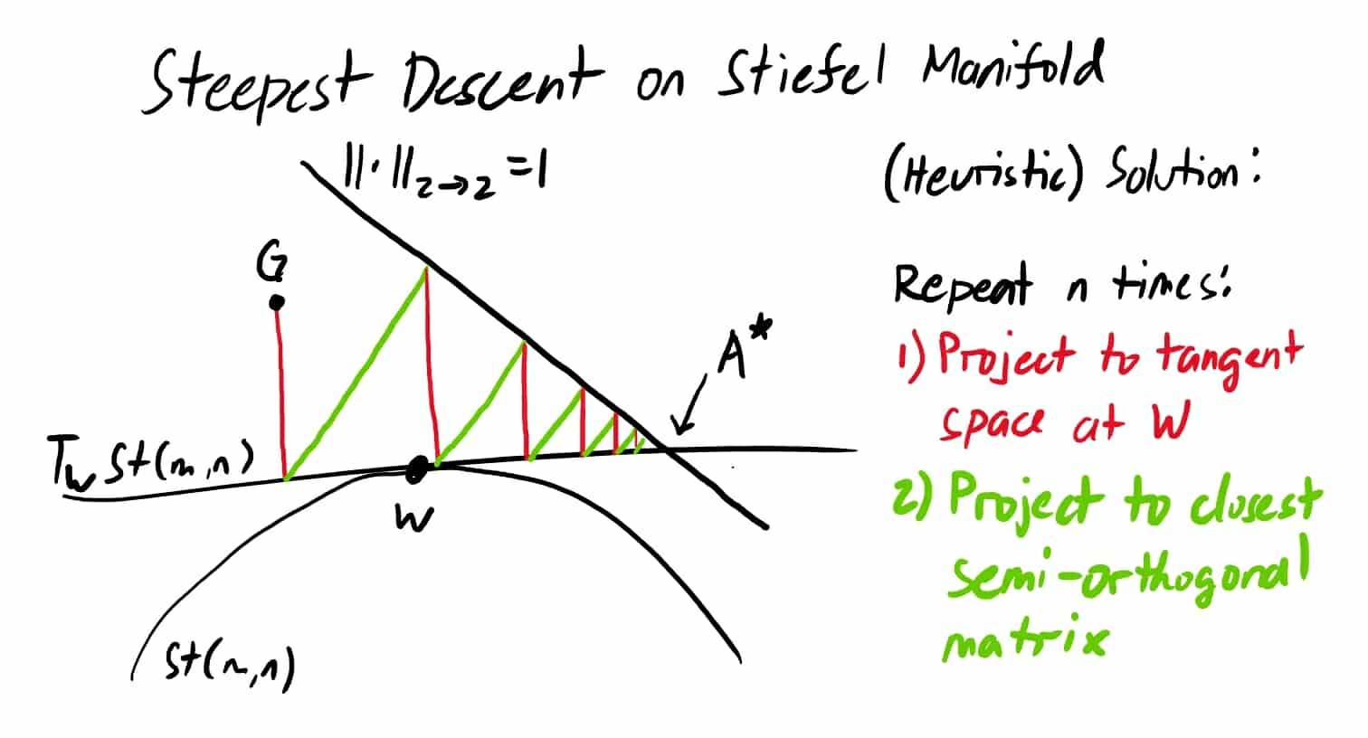
4. Projection-projection perspective
One can interpret Bernstein’s and Su’s solutions as a two-step projection process:
- (Orthogonal) projection to the tangent space at $W$; and
- Projection to the closest semi-orthogonal matrix (i.e., closest point on the Stiefel manifold).
This is because the map $G \to G - W \texttt{sym}(W^T G)$ is actually the orthogonal projection onto the tangent space at $W$ and that $\texttt{msign}$ projects the resulting matrix to the Stiefel manifold. We present these more rigorously as follows.
Theorem 2 (Orthogonal projection to the tangent space at $W$). Let $W \in \text{St}(m, n)$ be a point on the Stiefel manifold. The projection of a vector $V \in \mathbb{R}^{m \times n}$ onto the tangent space at $W$, denoted as $T_W\text{St}(m, n)$ , is given by,
$$\begin{equation} \texttt{proj}_{T_W\text{St}(m, n)}(V) = V - W \text{sym}(W^T V) \end{equation}$$
Proof. First, we need to show that the normal space at $W$, $N_W\text{St}(m, n)$ is given by, for symmetric $S$. To show this, let $A \in T_W\text{St}(m, n)$ be an arbitrary tangent vector at $W$. Then we have, Thus $\langle A, WS \rangle = 0$ which implies that $A$ and $WS$ are orthogonal. Hence $WS \in N_W\text{St}(m, n)$. Now, for any $V \in \mathbb{R}^{m \times n}$, we can write it as,
$V = \underbrace{V - WS}_{\text{candidate tangent}} + \underbrace{WS}_{\text{candidate normal}}$ for some symmetric $S$. To find $S$, Thus, $V - W \text{sym}(W^T V) \in T_W\text{St}(m, n)$. And because of that, $W^T (V - W \text{sym}(W^T V))$ must be skew-symmetric. Thus, Hence, $V - W \text{sym}(W^T V)$ is the orthogonal projection of $V$ onto the tangent space at $W$.Show proof of Theorem 2
And from Proposition 4 of Bernstein & Newhouse (2024),
Proposition 3 (Projection to the closest semi-orthogonal matrix). Consider the orthogonal matrices $\mathcal{O}_{m \times n} := \{ A \in \mathbb{R}^{m \times n} : A A^T = I_m or A^T A = I_n \}$ and let $\| \cdot \|_F$ denote the Frobenius norm. For any matrix $G \in R^{m \times n}$ with reduced SVD $G = U \Sigma V^T$:
$$\arg\min_{A \in \mathcal{O}_{m \times n}} \| A - G \|_F = \texttt{msign}(G) = UV^T,$$where the minimizer $UV^T$ is unique if and only if the matrix $G$ has full rank.
Thus we can write,
$$A^*_{\text{bernstein}} = A^*_{\text{su}} = (\texttt{proj}_{\text{St}(m, n)} \circ \texttt{proj}_{T_W\text{St}(m, n)})(G)$$for the square and full-rank case at least.
4.1. Why Bernstein’s & Su’s solutions only work for the square and full-rank case
Note that the projections above aim to guarantee both of our criteria for the solution, but one step at a time. And that the $\texttt{msign}$ after the projection may send the resulting matrix outside the tangent space at $W$. We show that this is not a problem in the square and full-rank case, but it is in the general case.
| operation | on the tangent space at $W$? | have unit spectral norm? |
|---|---|---|
| (input $G$) | not in general | not in general |
| 1st projection ($\texttt{proj}_{T_W St(m, n)}(\cdot)$) | ${\color{green}\text{yes}}$ | not necessarily |
| 2nd projection ($\texttt{msign}(\cdot$)) | only for the square and full-rank case | ${\color{green}\text{yes}}$ |
To demonstrate this, we will need the following proposition.
Proposition 4 ($\texttt{msign}$ preserves skew-symmetry). Let $X \in \mathbb{R}^{m \times n}$ be a skew-symmetric matrix. Then $\texttt{msign}(X)$ is also skew-symmetric.
The proof follows directly from the transpose equivariance and oddness of $\texttt{msign}$, i.e., $\texttt{msign}(X) = \texttt{msign}(-X^T) = -\texttt{msign}(X)^T$.
Also note that for the general case,
$$\begin{equation} WW^T + QQ^T = I_m \quad\text{and}\quad W^T Q = 0 \end{equation}$$where $Q$ is the orthonormal complement of $W$.
Thus,
$$\begin{align*} (\texttt{proj}_{\text{St}(m, n)} \circ \texttt{proj}_{T_W St(m, n)})(G) &= \texttt{msign}(G - \frac{1}{2}W W^T G - \frac{1}{2} W G^T W) \\ &= \texttt{msign}((WW^T + QQ^T)G - \frac{1}{2}W W^T G - \frac{1}{2} W G^T W) \\ &= \texttt{msign}(W \texttt{skew}(W^T G) + QQ^T G) \end{align*}$$For the square and full-rank case, we have $Q = 0$ and $W W^T = I$. And the above simplifies to Berstein’s solution,
$$(\texttt{proj}_{\text{St}(m, n)} \circ \texttt{proj}_{T_W St(m, n)})(G) = W \texttt{msign}(\texttt{skew}(W^T G))$$and since $\texttt{skew}(W^T G)$ is skew-symmetric, then $\texttt{msign}(\texttt{skew}(W^T G))$ must be too. And thus,
$$\begin{align*} &W^T (\texttt{proj}_{\text{St}(m, n)} \circ \texttt{proj}_{T_W St(m, n)})(G) + (\texttt{proj}_{\text{St}(m, n)} \circ \texttt{proj}_{T_W St(m, n)})(G)^T W \\ &\qquad= W^T W \texttt{msign}(\texttt{skew}(W^T G)) + (W\texttt{msign}(\texttt{skew}(W^T G)))^T W \\ &\qquad= \texttt{msign}(\texttt{skew}(W^T G)) + \texttt{msign}(\texttt{skew}(W^T G))^T \\ &\qquad= 0 \end{align*}$$Hence for the square and full-rank case, this two-step projection process guarantees that the resulting matrix has unit spectral norm and is in the tangent space at $W$.
For the more general case, we may no longer have $Q = 0$ or $W W^T = I$. Thus, we cannot guarantee that $W \texttt{skew}(W^T G) + QQ^T G$ is skew-symmetric. And so the $\texttt{msign}$ after the first projection may send the resulting matrix outside the tangent space at $W$.
5. Heuristic solutions for the general case
5.1. Alignment upper bound
As established previously, for any $G \in \mathbb{R}^{m \times n}$, the solution to $\arg\max_{A \in \text{St}(m, n)} \langle G, A \rangle$ is $A^* = \texttt{proj}_{\text{St}(m, n)}(G) = \texttt{msign}(G)$ and thus $\max_{A \in \text{St}(m, n)} \langle G, A \rangle = \| G \|_{\text{nuc}}$ where $\| \cdot \|_{\text{nuc}}$ is the nuclear norm. With an extra linear constraint $A \in T_W \text{St}(m, n)$, we have,
$$\begin{align*} \max_{A \in \text{St}(m, n) \cap T_W \text{St}(m, n)} \langle G, A \rangle &= \max_{A \in \text{St}(m, n) \cap T_W \text{St}(m, n)} \langle \underbrace{G - \texttt{proj}_{T_W \text{St}(m, n)}(G)}_{\in N_W\text{St}(m, n)} + \texttt{proj}_{T_W \text{St}(m, n)}(G), A \rangle \\ &= \max_{A \in \text{St}(m, n) \cap T_W \text{St}(m, n)} \langle \texttt{proj}_{T_W \text{St}(m, n)}(G), A \rangle \\ &\leq \max_{A \in \text{St}(m, n)} \langle \texttt{proj}_{T_W \text{St}(m, n)}(G), A \rangle \\ \max_{A \in \text{St}(m, n) \cap T_W \text{St}(m, n)} \langle G, A \rangle &\leq \| \texttt{proj}_{T_W \text{St}(m, n)}(G) \|_{\text{nuc}} \end{align*}$$The alignment between an element in the normal space and an element in the tangent space is always zero, i.e., $\langle \texttt{proj}_{T_W \text{St}(m, n)}(G), \texttt{proj}_{N_W \text{St}(m, n)}(G) \rangle = 0$. Thus, we can cancel out the first term in the first equality. And we have first inequality because the max over a smaller set is less than or equal to the max over a larger set.
We achieve equality in the square and full-rank case because the maximizer for the first inequality is guaranteed to be in the tangent space at $W$, as discussed in the previous section.
5.2. Fixed-point iteration of alternating projections
Notice that $QQ^T G$ is the projection of $G$ onto the column space of $Q$, $\texttt{proj}_{\text{col}(Q)}(G) = QQ^T G$. One can think of this as the component of $G$ that is, in a sense, not “aligned to” $W$. In practice, this is typically small relative to the component of $G$ that is “aligned to” $W$. If so, then,
$$(\texttt{proj}_{\text{St}(m, n)} \circ \texttt{proj}_{T_W St(m, n)})(G) \approx \texttt{msign}(W \texttt{skew}(W^T G) + \cancel{\texttt{proj}_{\text{col}(Q)}(G)}),$$which means that while the resulting matrix after the two projections may not be in the tangent space at $W$, it would likely be nearby. And repeating this process a few times should close the gap.
Sample implementation:
def project_to_stiefel_tangent_space(X, delta_X):
    return delta_X - X @ sym(X.T @ delta_X)

def orthogonalize(X):
    # copy Newton-Schulz iteration from Muon (Jordan et al., 2024)

def steepest_descent_stiefel_manifold_heuristic(W, G, num_steps=1):
    assert num_steps > 0, "Number of steps must be positive"
    A_star = G
    for _ in range(num_steps):
        A_star = project_to_stiefel_tangent_space(W, A_star)
        A_star = orthogonalize(A_star)
    return A_star
5.2.1. Local (linear) convergence guarantee
For now, we cannot yet guarantee global convergence as it would potentially require deriving the Lyapunov function for this iteration which is extremely difficult. What we can guarantee, however, is local convergence due to $\text{St}(m, n)$ and $T_W\text{St}(m, n)$ being closed semi-algebraic sets. That is, assuming that the initial point $W$ is “close enough” to the intersection, we can guarantee that a subsequence of the iterates converges to a point in the intersection. Furthermore, assuming transversality, we can guarantee that the convergence is linear.
Definition 5 (Semi-algebraic set) Let $\mathbb{F}$ be a real closed field. A subset $S$ of $\mathbb{F}^n$ is a semi-algebraic set if it is a finite union of sets defined by polynomial equations and inequalities.
We can construct $\text{St}(m, n) = \{ W \in \mathbb{R}^{m \times n} \| W^T W = I_n \}$ via $n(n+1)/2$ polynomial equations, and $T_W\text{St}(m, n) = \{ A \in \mathbb{R}^{m \times n} \| W^T A + A^T W = 0 \}$ via $mn$ polynomial equations. Hence both are semi-algebraic sets. And the intersection of two semi-algebraic sets is also a semi-algebraic set. From Theorem 7.3 of Drusvyatskiy et al. (2016), we then have the following convergence guarantee.
Theorem 6 (Convergence of alternating projections on semi-algebraic sets) Consider two nonempty closed semi-algebraic sets $X, Y \subset E$ with $X$ bounded. If the method of alternating projections starts in $Y$ and near $X$, then the distance of the iterates to the intersection $X \cap Y$ converges to zero, and hence every limit point lies in $X \cap Y$.
Setting $Y = T_W\text{St}(m, n)$, $X = \text{St}(m, n)$, and noting that the Stiefel manifold is bounded, we have that the iterates of our method of alternating projections converge to a point in the intersection $\text{St}(m, n) \cap T_W\text{St}(m, n)$.
But does this algorithm converge in sufficient time? Somewhat yes, we can guarantee local linear convergence assuming transversality.
Definition 7 (Transversality) Let $\mathcal{M}$ and $\mathcal{N}$ be two (smooth) manifolds in a Euclidean space. We say that $\mathcal{M}$ and $\mathcal{N}$ intersect transversally at a point $x \in \mathcal{M} \cap \mathcal{N}$ when,
$$N_x\mathcal{M} \cap N_x\mathcal{N} = \{0\}.$$
Intuitively speaking, this means that the tangent spaces at the intersection of the two manifolds have an “angle” between them, i.e., they are not parallel. The larger this angle is, the faster the convergence; and the smaller the angle, the slower the convergence. Theorem 2.1 of Drusvyatskiy et al. (2016) then gives us the following local linear convergence guarantee.
Theorem 8 (Linear convergence of alternating projections, assuming transversality) If two closed sets in a Euclidean space intersect transversally at a point $\tilde{x}$, then the method of alternating projections, started nearby, converges linearly to a point in the intersection.
$\text{St}(m, n)$ and $T_W\text{St}(m, n)$ are both closed sets so the theorem above applies.
5.3. Ternary search over nearby feasible solutions
Here we present an alternative solution that is more efficient, but often yields slightly more suboptimal results than the fixed-point iteration method above.
5.3.1. Problem decomposition
The crux is to split $\arg\max_{A\in \mathbb{R}^{m \times n}} \langle G, A \rangle$ into two optimization problems, one for the component of $G$ that is “aligned to” $W$ and one for the component of $G$ that is “not aligned to” $W$. To see this, let us first decompose $G$ and $A$ into,
$$G = W G_W + Q G_Q \qquad A = WB + QC$$where $G_W = W^T G$ and $G_Q = Q^T G$. Thus,
$$\begin{align} \langle G, A \rangle &= \langle W G_W + Q G_Q, WB + QC \rangle \nonumber \\ &= \text{tr}((W G_W + Q G_Q)^T (WB + QC)) \nonumber \\ &= \text{tr}(G_W^T B + G_Q^T C) \nonumber \\ \langle G, A \rangle &= \langle G_W, B \rangle + \langle G_Q, C \rangle \\ \end{align}$$The cross terms vanish in the third equality because $W^T Q = 0$. Finding the maximizer $A^*$ for the LHS is then equivalent to finding the maximizers $B^*$ and $C^*$ for the RHS and then combining them,
$$A^* = WB^* + QC^*.$$5.3.2. Solving the two subproblems
Now, to satisfy the constraint $A \in T_W\text{St}(m, n) \cap \text{St}(m, n)$,
$$\begin{align*} W^T A + A^T W &= 0 \qquad\qquad& A^T A &= I_n \\ W^T (WB + QC) + (WB + QC)^T W &= 0 \qquad\qquad& (WB + QC)^T(WB + QC) &= I_n \\ B + B^T &= 0 \qquad\qquad& B^T B + C^T C &= I_n \\ \end{align*}$$That is, we require that $B$ is skew-symmetric and $C$ satisfies $C^T C = I_n - B^T B$.
We cannot simply treat each subproblem separately because the second constraint couples $B$ and $C$. However, for this approximation, we make the assumption that doing so would yield a “good enough” solution.
For the first term, we can decompose $G_W$ into its skew-symmetric and symmetric components, $G_W = \texttt{skew}(G_W) + \texttt{sym}(G_W)$,
$$\begin{align*} \arg\max_{B \text{ is skew}} \langle G_W, B \rangle &= \arg\max_{B \text{ is skew}} \langle \texttt{skew}(G_W) + \texttt{sym}(G_W), B \rangle \\ &= \arg\max_{B \text{ is skew}} \langle \texttt{skew}(G_W), B \rangle + \cancel{\langle \texttt{sym}(G_W), B \rangle} \end{align*}$$And the maximizer is simply $\tilde{B} = \texttt{skew}(G_W) = \texttt{skew}(W^T G)$.
However, because of the constraint $B^T B + C^T C = I$, we have to “cap” the spectral norm of $B$ to be less than or equal to 1 otherwise we would fail to construct a real-valued $C$. We can do this via a variety of methods discussed in a previous post on spectral clipping and our latest paper on training transformers with enforced Lipschitz bounds (Newhouse*, Hess*, Cesista* et al., 2025). Let $\tau \leq 1$ be the spectral norm bound, then we can choose,
$$B^*(\tau) := \texttt{hardcap}_{\tau}(\tilde{B}) \quad\text{or}\quad B^*(\tau) := \tau\cdot\texttt{msign}(\tilde{B}) \quad\text{or}\quad B^*(\tau) := \frac{\tau}{\| \tilde{B} \|_{2 \to 2}}\tilde{B}$$These mappings preserve skew-symmetry and thus $B^*(\tau)$ satisfies the first constraint.
Now, parametrize $C$ as $C = UR$ where $U^T U = I$ and $R(\tau) = (I_n - (B^*(\tau))^T B^*(\tau))^{1/2}$. It is trivial to check that $C$ satisfies our constraints and that $R(\tau)$ is SPD. Thus, assuming we already have a fixed $B^*(\tau)$ (and consequently a fixed $R(\tau)$), solving the second subproblem,
$$\arg\max_{C} \langle G_Q, C \rangle$$is equivalent to solving,
$$\begin{align*} \arg\max_{U: U^T U = I} \langle G_Q, U R(\tau) \rangle &= \arg\max_{U: U^T U = I} \text{tr}(G_Q^T U R(\tau)) \\ &= \arg\max_{U: U^T U = I} \text{tr}(R(\tau) G_Q^T U) \\ &= \arg\max_{U: U^T U = I} \langle G_Q R(\tau), U \rangle \end{align*}$$which has maximizer $U^* = \texttt{msign}(G_Q R(\tau))$. Thus, $C^*(\tau) = \texttt{msign}(G_Q R(\tau)) R(\tau)$.
Note that for the square and full-rank case, we have $C = 0$ and so we require $B^T B = I$. For this, we can choose to orthogonalize $B = \texttt{skew}(G_W)$ which then yields Bernstein’s solution,
$$A^*_{\text{bernstein}} = W \texttt{msign}(\texttt{skew}(W^T G))$$This also motivates the choice of $\texttt{msign}$ as the normalization method for $B$ more generally.
We can implement this in JAX as follows,
from spectral_clipping import spectral_hardcap, spectral_normalize, orthogonalize

def matsqrt(W: jax.Array):
    # We can also compute this via Newton-Schulz iteration or Cholesky decomposition
    U, s, Vh = jnp.linalg.svd(W, full_matrices=False)
    s_sqrt = jnp.sqrt(s)
    return U @ jnp.diag(s_sqrt) @ Vh

def construct_nearby_feasible_solution(W, Q, G, tau=0.5, normalizer_method=0):
    m, n = W.shape
    if m == n:
        # assumes full-rank
        A = W @ orthogonalize(skew(W.T @ G))  # Bernstein's solution
    else:
        B = skew(W.T @ G)
        if normalizer_method == 0:
            B_tilde = tau * orthogonalize(B)
        elif normalizer_method == 1:
            B_tilde = spectral_hardcap(B, tau)
        elif normalizer_method == 2:
            B_tilde = spectral_normalize(B, tau)
        R = jnp.linalg.cholesky(jnp.eye(n) - B_tilde.T @ B_tilde)
        # R = matsqrt(jnp.eye(n) - B_tilde.T @ B_tilde)
        C = orthogonalize(Q.T @ G @ R) @ R
        A = W @ B_tilde + Q @ C
    return A
5.3.1. Where ternary search comes in

From Equation (7), we have,
$$\begin{align*} f(\tau) := \langle G, A^*(\tau) \rangle &= \langle G_W, B^*(\tau) \rangle + \langle G_Q, C^*(\tau) \rangle \\ &= \langle \texttt{skew}(G_W), B^*(\tau) \rangle + \langle G_Q, C^*(\tau) \rangle \\ &= \langle \texttt{skew}(G_W), \texttt{normalized}_{\tau}(\texttt{skew}(G_W)) \rangle + \langle G_Q, \texttt{msign}(G_Q R(\tau)) R(\tau) \rangle \\ &= \langle \texttt{skew}(G_W), \texttt{normalized}_{\tau}(\texttt{skew}(G_W)) \rangle + \| G_QR(\tau) \|_{\text{nuc}} \\ \end{align*}$$The first term is linear and positively-sloped as we vary $\tau$. And since the map $x \mapsto \sqrt{1 - x^2}$ is concave and non-increasing in $x \in [0, 1]$, the second term must be concave and non-increasing as we increase $\tau$. Taken together, $f$ must be unimodal. And thus we can use ternary search to find the optimal $\tau$ that maximizes $f(\tau)$.
We can implement this in JAX as follows,
def ternary_search_over_taus(W, Q, G, lo=0., hi=1., normalizer_method=0, max_iter=10):
    def evaluate(tau):
        A = construct_nearby_feasible_solution(W, Q, G, tau, normalizer_method)
        return jnp.trace(G.T @ A)

    def body_fun(i, val):
        lo, hi = val
        mid1 = (2*lo + hi) / 3
        mid2 = (lo + 2*hi) / 3
        f_mid1 = evaluate(mid1)
        f_mid2 = evaluate(mid2)
        new_lo = jnp.where(f_mid1 > f_mid2, lo, mid1)
        new_hi = jnp.where(f_mid1 > f_mid2, mid2, hi)
        return new_lo, new_hi
    final_lo, final_hi = jax.lax.fori_loop(0, max_iter, body_fun, (lo, hi))

    # Compute final midpoint and its value
    final_tau = (final_lo + final_hi) / 2
    final_value = evaluate(final_tau)
    return final_tau, final_value
6. Bonus: a Muon-like optimizer for the Embedding and Unembedding layers
Embedding layers have a hidden geometry: the (scaled-)Oblique manifold, $\widetilde{\text{Ob}}(m, n) = \{ W \in \mathbb{R}^{m \times n} \| \text{diag}(W^T W) = s^2\mathbf{1}_n \}$ with scale $s = \sqrt{m}$, or the manifold of matrices with unit-RMS-norm columns. More precisely, it is the embedding layer and the normalization layer right after it that results in unit-RMS-norm feature-vectors. But optimizers like Adam typically ignore this geometry and even its matrix-structure, treating the embedding layer the same as ‘flat’ vectors. We believe this leads to suboptimal performance and demonstrate this via grokking experiments we discuss in the next section.
What if we build an optimizer that respects this geometry?
For this, we need two things:
- A ‘dualizer’ map that maps a “raw gradient” matrix $G \in \mathbb{R}^{m \times n}$ to an update direction of steepest descent on the tangent space at $W \in \widetilde{\text{Ob}}(m, n)$, i.e., $A^* \in T_W\widetilde{\text{Ob}}(m, n)$ with $\| A^* \| = 1$ for some norm $\| \cdot \|$ chosen a priori. And,
- A ‘projection’ or retraction map that maps an (updated) weight matrix $W \in \mathbb{R}^{m \times n}$ back to the (scaled-)Oblique manifold.
The retraction map is simply the column-wise normalization,
$$\texttt{col\_normalize}(W) := \text{col}_j(W) \mapsto \frac{\text{col}_j(W)}{\| \text{col}_j(W) \|_{RMS}} = \sqrt{m}\frac{\text{col}_j(W)}{\| \text{col}_j(W) \|_{2}} \quad \forall 0 \leq j < n$$where $\text{col}_j(W)$ is the $j$-th column of the weight matrix $W$.
As for the dualizer, which norm should we use? We can, for example, use the RMS-to-RMS norm for consistency and still be able to use the same alternating projection method as before. However, as argued by Bernstein & Newhouse (2024) and Pethick et al. (2024), it may be more natural to use the L1-to-RMS norm, $\| \cdot \|_{1\to RMS}$ because the maximizer for the following problem,
$$\arg\max_{A: \| A \|_{1 \to RMS} = 1} \langle G, A \rangle$$is simply $\texttt{col\_normalize}(G) \in \widetilde{\text{Ob}}(m, n)$. That is, all of the token embedding updates would have the same size, improving training stability. Thus our update rule becomes,
$$ W \leftarrow \texttt{col\_normalize}(W - \eta A^*)$$where $\eta$ is the learning rate and,
$$ A^* = \arg\max_{A: \| A \|_{1 \to RMS} = 1} \langle G, A \rangle \quad \text{s.t. } A \in T_W\widetilde{\text{Ob}}(m, n),$$Equivalently,
$$A^* = \arg\max_{A} \langle G, A \rangle \quad \text{s.t. } A \in \widetilde{\text{Ob}}(m, n) \cap T_W \widetilde{\text{Ob}}(m, n),$$or in words, we want to find a descent direction $A^*$ that is both on the (scaled-)Oblique manifold and in the tangent space at $W$ that maximizes the alignment with the “raw gradient” $G$.
6.1. Optimal solution for steepest descent on the (scaled-)Oblique manifold
The Oblique manifold is a product of hyperspheres, $\text{Ob}(m, n) = \underbrace{S^m \times \ldots \times S^m}_{n}$. So, in a sense, the columns are acting independently of each other and steepest descent on the Oblique manifold is equivalent to steepest descent on the hypersphere, applied column-wise. Generalizing Bernstein’s (2025b) dualizer for steepest descent on the hypersphere to the Oblique manifold then yields,
The optimal solution for finding the direction of steepest descent on the Oblique manifold $A^*$ given “raw Euclidean gradient” or differential $G$ is to simply project $G$ onto the tangent space at point $W \in \widetilde{\text{Ob}}(m, n)$ and then normalize column-wise.
The tangent space at $W$ is simply,
$$T_W\widetilde{\text{Ob}}(m, n) = \{A \in \mathbb{R}^{m \times n} \| \text{diag}(W^T A) = 0\}$$or in words, the column-wise dot-product or “alignment” between $W$ and a candidate tangent vector $A$ must be zero for $A$ to be in the tangent space at $W$. The projector onto the tangent space at $W$ is then given by,
$$\texttt{proj}_{T_W\widetilde{\text{Ob}}(m, n)}(G) = G - W \text{diag}(W^T G / m)$$or in words, we subtract the component of $G$ that is “aligned to” $W$.
Notice then that one of the constraints is concerned with the size of the columns while the other is concerned with the direction. These can be optimized independently of each other. Thus, the solution for $A^*$ is then simply,
$$A^* = \texttt{col\_normalize}(\texttt{proj}_{T_W\widetilde{\text{Ob}}(m, n)}(G))$$6.2. Steepest descent on the (scaled-)Row-Oblique manifold
We argue that the Unembedding layer or the ’language model head’ should naturally be on the (scaled-)Row-Oblique manifold, $\widetilde{\text{RowOb}}(m, n) = \{ W \in \mathbb{R}^{m \times n} | \text{diag}(WW^T) = s^2\mathbf{1}_m \}$ with scale $s = \sqrt{n}$, or the manifold of matrices with unit-RMS-norm rows. The crux is that the logit for the $i$-th vocabulary token is given by the dot-product or ‘alignment’ between the $i$-th row of the weight matrix and the feature vector. So if the logits measure ‘alignment’, not ‘size’, then it is natural to constrain the rows to have unit-RMS-norm.
And since we can construct $\widetilde{\text{RowOb}}(m, n)$ by transposing $\widetilde{\text{Ob}}(m, n)$, we can use the same reasoning as above to derive the optimal solution for steepest descent on the (scaled-)Row-Oblique manifold.
Our retraction map is simply the row-wise normalization,
$$\texttt{row\_normalize}(W) := \text{row}_i(W) \mapsto \frac{\text{row}_i(W)}{\| \text{row}_i(W) \|_{RMS}} = \sqrt{n}\frac{\text{row}_i(W)}{\| \text{row}_i(W) \|_{2}} \quad \forall 0 \leq i < m$$where $\text{row}_i(W)$ is the $i$-th row of the weight matrix $W$. We then choose the $\| \cdot \|_{RMS \to \infty}$ norm because the maximizer for the following problem,
$$\arg\max_{A: \| A \|_{RMS \to \infty} = 1} \langle G, A \rangle$$is simply $\texttt{row\_normalize}(G) \in \widetilde{\text{RowOb}}(m, n)$. That is, the per-row updates would have even size.
Our update rule then becomes,
$$ W \leftarrow \texttt{row\_normalize}(W - \eta A^*)$$where $\eta$ is the learning rate and,
$$A^* = \arg\max_{A} \langle G, A \rangle \quad \text{s.t. } A \in \widetilde{\text{RowOb}}(m, n) \cap T_W \widetilde{\text{RowOb}}(m, n),$$which has the closed form solution,
$$\begin{align*} A^* &= \texttt{row\_normalize}(\texttt{proj}_{T_W\widetilde{\text{RowOb}}(m, n)}(G)) \\ &= \texttt{row\_normalize}(G - \text{diag}(G W^T / n) W) \\ \end{align*}$$7. Experimental results
7.1. Alternating projections method beats ternary search on nearby feasible solutions on larger matrices


Here we compare our two heuristic methods for the problem of spectral-norm constrained steepest descent on the Stiefel manifold. Observe from the figures above that the ternary search over nearby feasible solutions method results in almost optimal solutions, regardless of scale. However, the alternating projections method results in more aligned solutions, albeit at the cost of more compute and being more off-tangent.
7.2. Grokking on the Addition-Modulo-113 task in 44 full-batch training steps
We will release the source code soon, but if you want early access, please email me.

We use the same training setup for grokking experiments on the Addition-Modulo-113 problem as in a previous post on spectral clipping, with new dualizers and projection maps added. Following Prieto et al. (2025), we use a 2-layer MLP (plus Embedding and Unembedding layers) with 200 hidden units per layer. All matrix multiplications are done in bfloat16 precision.
We place our Embedding and Unembedding weights on the (scaled-)Oblique manifold and (scaled-)Row-Oblique manifold, respectively. We then vary the dualizer and retraction maps used in the linear layers and report the best median-steps-to-grokking across 64 random seeds. See figure above for the results.
Interestingly, without weight constraints, models fail to grok within 1000 full-batch training steps. This is true for both the Muon optimizer and AdamW. However, with weight constraints, we were able to achieve grokking in 44 full-batch training steps, which we believe is SOTA.
The best recipe seems to be:
| layer | manifold | $\texttt{dualizer}$ | $\texttt{retract}$ |
|---|---|---|---|
| Embedding | (Scaled-)Oblique manifold | $\texttt{col\_normalize} \circ \texttt{proj}_{T_W\widetilde{\text{Ob}}(m, n)}$ | $\texttt{col\_normalize}$ |
| 1st Linear | RMS-to-RMS norm ball around the origin of $\mathbb{R}^{m \times n}$ | $\texttt{msign}$ | $\texttt{spectral\_normalize}$ |
| 2nd Linear | RMS-to-RMS norm ball around the origin of $\mathbb{R}^{m \times n}$ | $\texttt{msign}$ | $\texttt{spectral\_normalize}$ |
| Unembedding | (Scaled-)Row-Oblique manifold | $\texttt{row\_normalize} \circ \texttt{proj}_{T_W\widetilde{\text{RowOb}}(m, n)}$ | $\texttt{row\_normalize}$ |
Acknowledgements
Big thanks to Jianlin Su, Jeremy Bernstein, Vinay Rao, Antonio Silveti-Falls, Mikail Khona, Omead Pooladzandi, Simo Ryu, and Kevin Yin for productive discussions on the topic. All remaining mistakes are mine.
How to cite
@misc{cesista2025spectralclipping,
  author = {Franz Louis Cesista},
  title = {{H}euristic Solutions for {S}teepest {D}escent on the {S}tiefel manifold},
  year = {2025},
  month = {July},
  day = {18},
  url = {https://leloykun.github.io/ponder/steepest-descent-stiefel/},
}
If you find this post useful, please consider supporting my work by sponsoring me on GitHub:
References
- Keller Jordan, Yuchen Jin, Vlado Boza, Jiacheng You, Franz Cesista, Laker Newhouse, and Jeremy Bernstein (2024). Muon: An optimizer for hidden layers in neural networks. Available at: https://kellerjordan.github.io/posts/muon/
- Greg Yang, James B. Simon, Jeremy Bernstein (2024). A Spectral Condition for Feature Learning. URL https://arxiv.org/abs/2310.17813
- Tim Large, Yang Liu, Minyoung Huh, Hyojin Bahng, Phillip Isola, Jeremy Bernstein (2024). Scalable Optimization in the Modular Norm. URL https://arxiv.org/abs/2405.14813
- Jeremy Bernstein, Laker Newhouse (2024). Old Optimizer, New Norm: An Anthology. URL https://arxiv.org/abs/2409.20325
- Laker Newhouse (2025). Understanding Muon. URL https://www.lakernewhouse.com/writing/muon-1
- Laker Newhouse, Preston Hess, Franz Cesista, Andrii Zahorodnii, Jeremy Bernstein, Phillip Isola (2025). Training Transformers with Enforced Lipschitz Constants. URL https://arxiv.org/abs/2507.13338
- Jeremy Bernstein (2025a). Orthogonal manifold. URL https://docs.modula.systems/algorithms/manifold/orthogonal/
- Jeremy Bernstein (2025b). Hypersphere. URL https://docs.modula.systems/algorithms/manifold/hypersphere/
- Jianlin Su (2025). Steepest descent on Stiefel manifold. URL https://x.com/YouJiacheng/status/1945522729161224532
- D. Drusvyatskiy, A.D. Ioffe, A.S. Lewis (2016). Transversality and alternating projections for nonconvex sets. URL https://arxiv.org/abs/1401.7569
- Thomas Pethick, Wanyun Xie, Kimon Antonakopoulos, Zhenyu Zhu, Antonio Silveti-Falls, Volkan Cevher (2025). Training Deep Learning Models with Norm-Constrained LMOs. URL https://arxiv.org/abs/2502.07529
- Bin Gao, Simon Vary, Pierre Ablin, P.-A. Absil (2022). Optimization flows landing on the Stiefel manifold. URL https://arxiv.org/abs/2202.09058
- Pierre Ablin, Gabriel Peyré (2021). Fast and accurate optimization on the orthogonal manifold without retraction. URL https://arxiv.org/abs/2102.07432
- Lucas Prieto, Melih Barsbey, Pedro A.M. Mediano, Tolga Birdal (2025). Grokking at the Edge of Numerical Stability. URL https://arxiv.org/abs/2501.04697